How does {multicolor} actually work?
- 2018/19/07
- 12 min read
Today in R/mildlyinteresting…the multicolor package! It’s built on Gábor Csárdi’s crayon for use in conjunction with Scott Chamberlain’s cowsay. Here’s an example of what it does.
library(multicolor)multi_color(things[["buffalo"]])
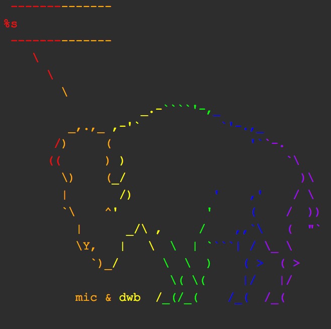
So yeah, mostly useless! But if you’re interested in how it works, I’ll take it apart and show you the parts that matter.
Background
The idea came about after I submitted a pull request to cowsay adding the ability to add a single color to the output of a call to cowsay::say. In other words, you could turn your entire cat spouting your error message in a package red, if you wanted. After some discussion with Scott about other ways we could add color, I suggested offering users a “rainbow” option.
When I submitted the PR I knew virtually nothing about how colors are applied to the text that shows up in your terminal or console. Poking through crayon taught me a bit about how colors work. I ended up taking a tidyverse-centric approach to make the multicoloring idea work such that multicolor::multi_color allows users to evenly apply any number of colors to any ASCII art animal they might want to print.
This post will talk through how multi_color (or if you prefer, multi_colour 😆) and text coloring in general works. If you have ideas for how to make the algorithm more efficient, get at me!
What is this cowsay you speak of
The cowsay package offers a fun way to deliver messages in packages that draw attention to themselves and ensure that the user sees them. For instance,
important_message <- "This option is only available with purrr >= 0.2.1"

say(what = important_message,
    by = "egret")
##
## -----
## This option is only available with purrr >= 0.2.1
## ------
## \
## \
## \
## \ _,
## -==<' `
## ) /
## / (_.
## | ,-,`\
## \\ \ \
## `\, \ \
## ||\ \`|,
## jgs _|| `=`-'
## ~~`~`The cowsay default is to message the input, but you can optionally print the bare string with type = "string". This bare string is just simple text including the backslash escapes and newlines needed to make it show up correctly in the R console.
cow_string <- say("moooooo",
                  by = "cow",
                  type = "string")
cow_string
## [1] "\n ----- \nmoooooo \n ------ \n \\ ^__^ \n \\ (oo)\\ ________ \n (__)\\ )\\ /\\ \n ||------w|\n || ||"Wrapping that string in cat, message, warning, or stop prints a character vector so it emerges into its full animal glory.
cat(cow_string)##
## -----
## moooooo
## ------
## \ ^__^
## \ (oo)\ ________
## (__)\ )\ /\
## ||------w|
## || ||warning(cow_string)## Warning:
## -----
## moooooo
## ------
## \ ^__^
## \ (oo)\ ________
## (__)\ )\ /\
## ||------w|
## || ||Also handily, the 42 strings that make up the animals and characters are stored in a named vector and exported, so they can be accessed with can be accessed with cowsay::animals. (They’re also exported in multicolor as multicolor::things.)
How cowsay::say works
Before getting into how color can be applied in an even fashion to cowsay animals, it’ll be useful to take a look into how cowsay works in the fist place.
The original cowsay::say that I came to takes two main arguments: what (the text the animal should say) and by (who should say it). say first assembles the entire string output by sprintfing the text the user wants the animal to say into the animal’s speech bubble. Then, depending on the type argument the user supplies, the whole thing is delivered as either the bare string or wrapped in message or warning. This works like:
## some stuff to determine our `what` and `by`

## create the string
full_string <- sprintf(by, what)

## message, warn, or print the string
switch(type,
       message = message(full_string),
       warning = warning(full_string),
       string = full_string)
Since the cowsay animals are some of the most expressive strings you’d print to your console, it seemed like a natural idea to bring color to them.
Okay so how about this crayon?
The tidyverse makes liberal use of the crayon package for coloring strings. I find it useful when running tests (green means good, red means bad, blue means skipped) or even just printing tibbles (red for NA, gray generally for metadata, etc.). Color provides a nice cognitive shortcut when scanning through bunches of information and also, it’s just cool.
crayon makes it very easy to add color to text by supplying and allowing users to create functions of class crayon. As an example of a built-in functiion, cat(crayon::blue("foo")), as you might expect, prints a blue “foo”. As with cowsay, printing the text directly prints the bare string, which can be cated, messageded, etc. into a character vector.
crayon::blue("foo")"\033[34mfoo\033[39m"If we take a look at what the function blue is doing, we see it’s attaching a sequence of tags to the beginning and the end of the text. Everything between those tags gets the style attached. green attaches slightly different tags.
crayon::green("bar")"\033[32mbar\033[39m"crayon also allows for the combination of multiple styles with the $ syntax. Styles prefixed with bg mean background.
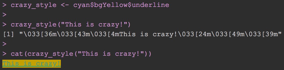
How to add color to animals?
These built-in crayon color functions are not flexible because they each only do one thing, but crayon provides a straightforward yet powerful way of creating user-defined colors in the make_style function.
make_style accepts a character vector which can be any of the grDevices::colors() or a hex value which can be generated from grDevices::rgb(). Then make_style creates a new function that, when called, will attach the correct opening and closing color tags to its argument. For instance:
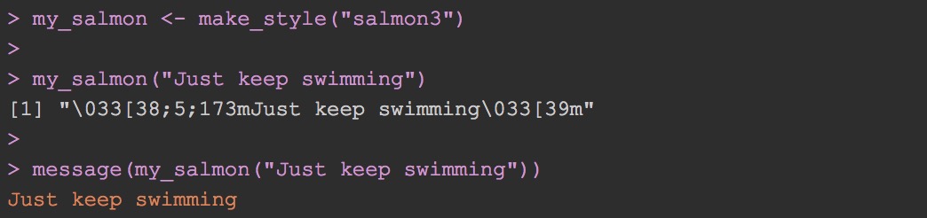
What this means is that we can use to for programming because it can color some arbitrary text any arbitrary color. We can accept a color string, feed it to make_style to create a function, and wrap our text in that function.
Evenly applying color
The crayon package offers a nice interface for applying multiple colors to text with the %+% operator but requires that users define the boundaries of those colors themselves. That won’t work for our goal of evenly applying any number of colors to any string; we need to programatically find out where those boundaries are so that we can insert color tags without needing to calculate where the red ends and the orange starts and so on.
This is a simpler problem when text is a single line, but a bit more complicated when it’s spread out over multiple lines as it is for the cowsay animals. The approach I ended up taking relies heavily on the tidyverse packages dplyr, tidyr, and purrr.
Main idea
The crux of how multi_color works is focused on correctly figuring out how to color the line with the greatest number of characters (call it longest_line_chars characters) by splitting it into the number of colors supplied (call that n_buckets buckets).
I’ll demonstrate on this chicken.
chicken <- cowsay::animals[["chicken"]]
cat(chicken)
##
##
## -----
## %s
## ------
## \
## \
## _
## _/ }
## `>' \
## `| \
## | /'-. .-.
## \' ';`--' .'
## \'. `'-./
## '.`-..-;`
## `;-..'
## _| _|
## /` /` [nosig]
## We split the chicken (chicken is being a very good sport about this) into each line and find the line with the greatest number of characters.
chicken_split <- chicken %>%
  stringr::str_split("\\n") %>%
  `[[`(1)

(longest_line <- chicken_split[which(nchar(chicken_split) ==
                      max(nchar(chicken_split)))])
## [1] " /` /` [nosig]"This longest_line should get split into evenish buckets of color.
If our colors are
our_colors <- c("honeydew2", "deepskyblue", "burlywood3")
n_buckets <- length(our_colors)
and our longest line has
(longest_line_chars <-
  nchar(longest_line))
## [1] 25characters in it, then we can chop those 25 into our n_buckets buckets of colors. I say roughly equal buckets our longest_line_chars (25 in this case) is not always divisible by n_buckets (3, here).
cut(seq(longest_line_chars),
    breaks = n_buckets,
      include.lowest = TRUE,
      dig.lab = 0
    ) %>%
    as.numeric()
## [1] 1 1 1 1 1 1 1 1 1 2 2 2 2 2 2 2 2 3 3 3 3 3 3 3 3If we had 7 colors instead of 3, then this would look like
cut(seq(longest_line_chars), 7,
      include.lowest = TRUE,
      dig.lab = 0
    ) %>%
    as.numeric()
## [1] 1 1 1 1 2 2 2 3 3 3 3 4 4 4 5 5 5 5 6 6 6 7 7 7 7Now we have the sequence of colors applied to every character in longest_line. This means we also know how to color every possible character index in our txt. Because we evenly apply colors vertically across the entire input, whatever color the 5th character in longest_line is will also be the same color as the 5th character (if it exists) in every other line. So by figuring out what longest_line looks like first, we can apply the same color pattern to every other line.
Actual Implementation 👩🎨
Above we have the key idea behind multi_color. The approach I took (after a few missteps 😂) was to keep everything we need in tidy dataframes that are joined on each other and unnested as necessary.
Like in the chicken example, we unpack the original string into individual lines, unpack those lines into characters, and assign each character the correct color. Then to actually apply a given color to a swath of characters, all we need to do is put the color’s opening tag before the first character and the closing tag after the last character in that swath1.
In a nutshell, the way this is actually implemented in multi_color is like this (should be decently well commented in the function):
- Define a helper function
get_open_closethat makes use of the internalcrayonfunctioncrayon:::style_from_r_colorfor looking up the opening and closing tags for a given color. (This takes care of all the hard work of looking up the correct tags, and works for both color strings like"lemonchiffon4"and hex values like"#66801A".) - Create a dataframe of each color supplied to
colorsalong with a unique identifier for it (important if the same color is supplied twice) and that color’s open tag and close tag - Make a separate tibble from the input
txt, splitting on the newlines to get one line per row, and a count of the number of characters in each line - Find the line with the max number of characters; this is the row that we’ll base all of the color assignments off of
- Cut the longest line into roughly equal buckets
- Assign a color for every possible character index based on the longest line. In other words, if the bucket size is 5, characters 1 through 5 are red, 5 through 10 are orange, etc.
- Create a list column housing the line split into individual characters and unnest it. Now we have a long dataframe where each row is an single character
- Assign a color to every character based on its position in the line
- Assign an
"open"flag to the characters that are the first of their color in the line and a"close"flag to characters that are the last of their color - Join this on the dataframe defining each color’s opening and closing tags. Now we have characters in the same row as the tags that will be attached to them
- For rows that have tags, concatenate open tags before the character and close tags after
- Add a newline after every row (since we split on
"\n"which removed them, we need to get these back in) - Collapse the entire output column into a string
Then we’re basically done!
Tags get applied like
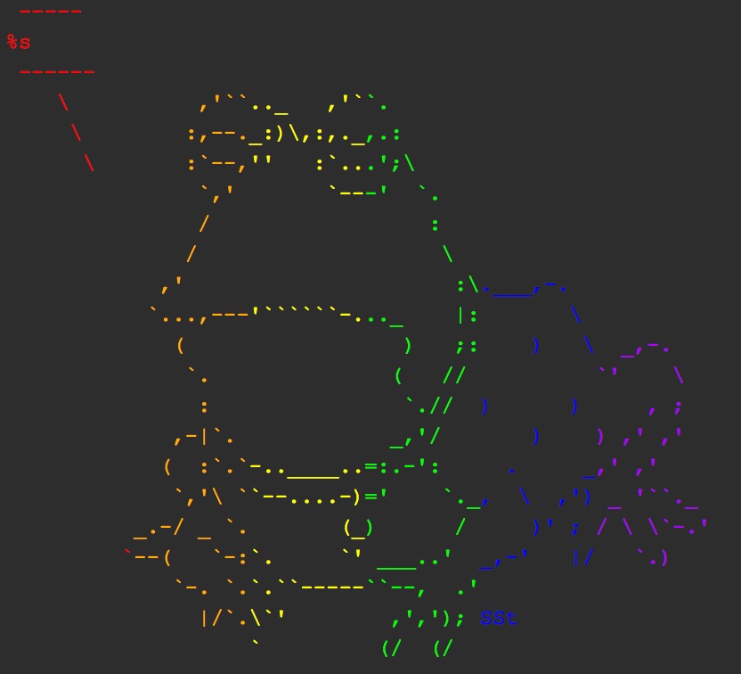
multi_color(things[["hypnotoad"]])## [38;5;196m ----- [39m
## [38;5;196m%s [39m
## [38;5;196m ------[39m
## [38;5;196m \ [39m[38;5;214m ,'``[39m[38;5;226m.._ ,'`[39m[38;5;46m`.[39m
## [38;5;196m \ [39m[38;5;214m :,--.[39m[38;5;226m_:)\,:,._[39m[38;5;46m,.:[39m
## [38;5;196m \ [39m[38;5;214m :`--,[39m[38;5;226m'' :`..[39m[38;5;46m.';\[39m
## [38;5;196m [39m[38;5;214m `,' [39m[38;5;226m `--[39m[38;5;46m-' `.[39m
## [38;5;196m [39m[38;5;214m / [39m[38;5;226m [39m[38;5;46m :[39m
## [38;5;196m [39m[38;5;214m / [39m[38;5;226m [39m[38;5;46m \[39m
## [38;5;196m [39m[38;5;214m ,' [39m[38;5;226m [39m[38;5;46m :\[39m[38;5;21m.___,-.[39m
## [38;5;196m [39m[38;5;214m `...,---[39m[38;5;226m'``````-.[39m[38;5;46m.._ |:[39m[38;5;21m \[39m
## [38;5;196m [39m[38;5;214m ( [39m[38;5;226m [39m[38;5;46m ) ;:[39m[38;5;21m ) \[39m[38;5;129m _,-.[39m
## [38;5;196m [39m[38;5;214m `. [39m[38;5;226m [39m[38;5;46m ( // [39m[38;5;21m [39m[38;5;129m`' \[39m
## [38;5;196m [39m[38;5;214m : [39m[38;5;226m [39m[38;5;46m `.// [39m[38;5;21m) ) [39m[38;5;129m , ;[39m
## [38;5;196m [39m[38;5;214m ,-|`. [39m[38;5;226m [39m[38;5;46m _,'/ [39m[38;5;21m ) [39m[38;5;129m) ,' ,'[39m
## [38;5;196m [39m[38;5;214m ( :`.`[39m[38;5;226m-..____..[39m[38;5;46m=:.-': [39m[38;5;21m . _[39m[38;5;129m,' ,'[39m
## [38;5;196m [39m[38;5;214m `,'\ `[39m[38;5;226m`--....-)[39m[38;5;46m=' `._[39m[38;5;21m, \ ,')[39m[38;5;129m _ '``._[39m
## [38;5;196m [39m[38;5;214m_.-/ _ `.[39m[38;5;226m (_[39m[38;5;46m) / [39m[38;5;21m )' ; [39m[38;5;129m/ \ \`-.'[39m
## [38;5;196m `[39m[38;5;214m--( `-:[39m[38;5;226m`. `'[39m[38;5;46m ___..' [39m[38;5;21m_,-' |/[39m[38;5;129m `.)[39m
## [38;5;196m [39m[38;5;214m `-. `.[39m[38;5;226m`.``-----[39m[38;5;46m``--, .'[39m
## [38;5;196m [39m[38;5;214m |/`.[39m[38;5;226m\`' [39m[38;5;46m ,','); [39m[38;5;21mSSt[39m
## [38;5;196m [39m[38;5;214m [39m[38;5;226m` [39m[38;5;46m (/ (/[39m
## [38;5;196m [39mand rendered like
If the user wants a message or warning, we wrap the output string in a message or warning function – same as the cowsay approach.
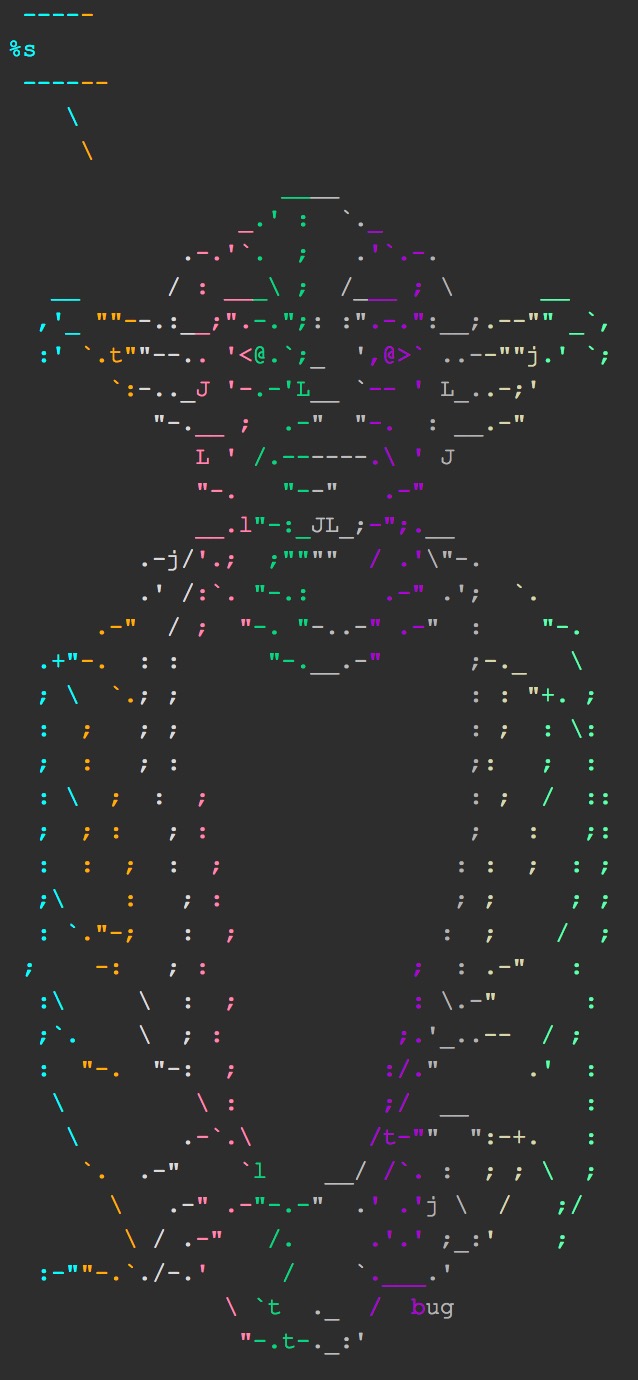
The tidyverse functions used in multi_color are fast enough that I haven’t found any reason to do any re-architecting or optimizing. It performs pretty well even for a big chunk of text like Yoda here.
multi_color(things[["yoda"]],
            colors = sample(colors(), 10)) %>%  # Randomly sample 10 colors
  bench::mark() %>%  # Jim Hester's new `bench` package!
  dplyr::select(min, mean, median, max)
## # A tibble: 1 x 4
## min mean median max
## <bch:tm> <bch:tm> <bch:tm> <bch:tm>
## 1 11ns 36.8ns 29ns 78.9µs
Wrap-up
That’s about it! You can mess around with coloring the cowsay animals which are exported in multicolor::things, but if you want to make them say anything you’ll need to use cowsay. When multiple colors are supplied to say, cowsay calls multi_color to handle the multicoloring. Otherwise, it just uses crayon to do its coloring.
For example,
say(what = "Fish are friends, not food",
    by = "shark",
    what_color = c("burlywood", "plum2", "burlywood"),
    by_color = c("aquamarine2", "peachpuff3", "limegreen"))
Happy coloring 🎨!
I first started off creating a
multi_colorfunction by individually coloring each character. That approach is slower and requires more color tags than are needed, since we only need an opening color tag at the beginning of each color boundary and a closing one at the end.↩