Catching Kareem
- 2018/13/06
- 12 min read
Lighting round of basketball analysis!
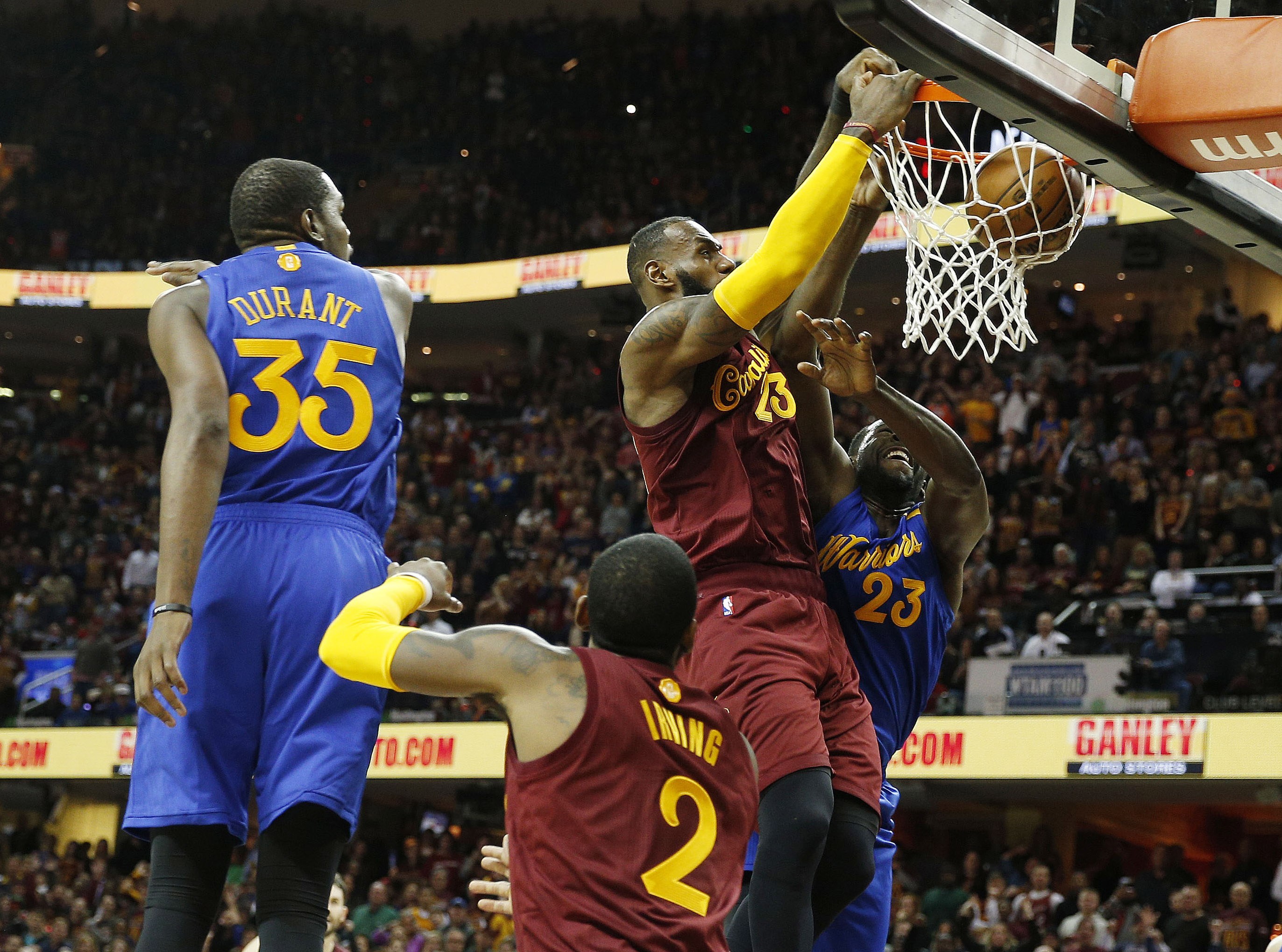
My friend and coworker Brad, who designed this very blog, is a sports fan and curious person. He wanted to know whether Lebron James is on track to overtake NBA all-time high scorer Kareem Abdul-Jabbar (38,387 career points!) in average number of points scored per game. He threw Kevin Durant in as a third point of comparison.
So our question is: who’s on track to unseat Kareem?
library(here)
library(tidyverse)
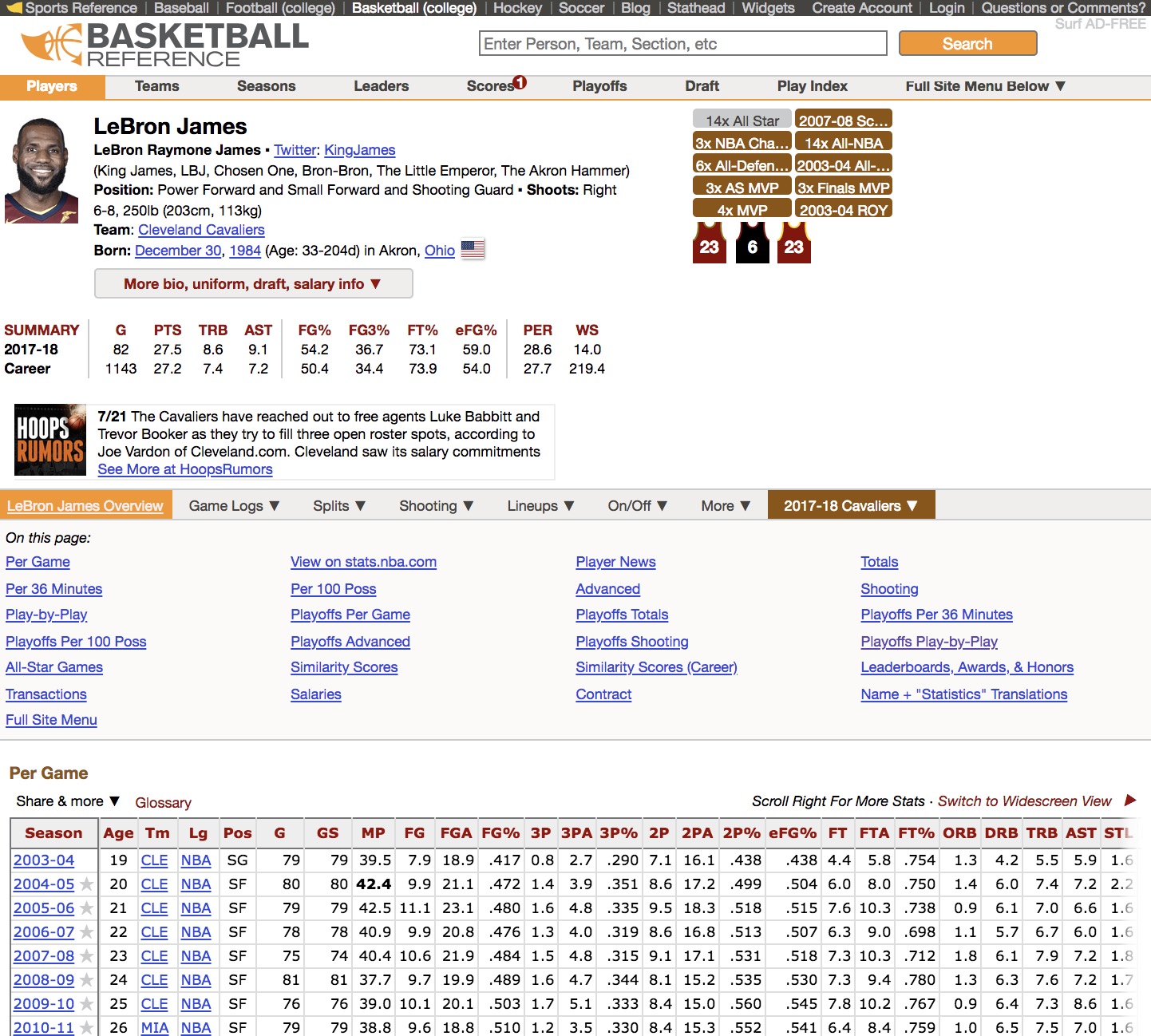
library(rvest) We’ll use Basketball Reference which apparently is an authority on these sorts of things.
There’s no way to download data as far as I could tell, so a quick check that we can scrape some of their tables.
robotstxt::paths_allowed("https://www.basketball-reference.com/")##
www.basketball-reference.com## [1] TRUEGetting Data
Each player on Basketball Reference here has their own page.
So for our three guys let’s stick their urls and names in two few character vectors.
kareem <- "https://www.basketball-reference.com/players/a/abdulka01.html"
lebron <- "https://www.basketball-reference.com/players/j/jamesle01.html"
durant <- "https://www.basketball-reference.com/players/d/duranke01.html"

player_urls <- c(kareem, lebron, durant)
player_names <- c("Kareem", "Lebron", "Durant")
Now we can scrape each url using rvest and the HTML tag table and throw it in a named list, giving it the name nsm[i], i.e. the player’s name we defined in player_names.
get_tables <- function(nms = player_names,
                       urls = player_urls) {
  out <- NULL

  for (i in seq_along(urls)) {
    this <-
      read_html(urls[i]) %>%
      html_nodes("table") %>%
      html_table()

    names(this) <- nms[i]

    out <- out %>% append(this)
  }
  return(out)
}
Let’s save that in an all_stats list
all_stats <- get_tables()glimpse(all_stats)## List of 3
## $ Kareem:'data.frame': 24 obs. of 30 variables:
## ..$ Season: chr [1:24] "1969-70" "1970-71" "1971-72" "1972-73" ...
## ..$ Age : int [1:24] 22 23 24 25 26 27 28 29 30 31 ...
## ..$ Tm : chr [1:24] "MIL" "MIL" "MIL" "MIL" ...
## ..$ Lg : chr [1:24] "NBA" "NBA" "NBA" "NBA" ...
## ..$ Pos : chr [1:24] "C" "C" "C" "C" ...
## ..$ G : int [1:24] 82 82 81 76 81 65 82 82 62 80 ...
## ..$ GS : int [1:24] NA NA NA NA NA NA NA NA NA NA ...
## ..$ MP : num [1:24] 43.1 40.1 44.2 42.8 43.8 42.3 41.2 36.8 36.5 39.5 ...
## ..$ FG : num [1:24] 11.4 13 14.3 12.9 11.7 12.5 11.1 10.8 10.7 9.7 ...
## ..$ FGA : num [1:24] 22.1 22.5 24.9 23.3 21.7 24.4 21.1 18.7 19.4 16.8 ...
## ..$ FG% : num [1:24] 0.518 0.577 0.574 0.554 0.539 0.513 0.529 0.579 0.55 0.577 ...
## ..$ 3P : num [1:24] NA NA NA NA NA NA NA NA NA NA ...
## ..$ 3PA : num [1:24] NA NA NA NA NA NA NA NA NA NA ...
## ..$ 3P% : num [1:24] NA NA NA NA NA NA NA NA NA NA ...
## ..$ 2P : num [1:24] 11.4 13 14.3 12.9 11.7 12.5 11.1 10.8 10.7 9.7 ...
## ..$ 2PA : num [1:24] 22.1 22.5 24.9 23.3 21.7 24.4 21.1 18.7 19.4 16.8 ...
## ..$ 2P% : num [1:24] 0.518 0.577 0.574 0.554 0.539 0.513 0.529 0.579 0.55 0.577 ...
## ..$ eFG% : num [1:24] 0.518 0.577 0.574 0.554 0.539 0.513 0.529 0.579 0.55 0.577 ...
## ..$ FT : num [1:24] 5.9 5.7 6.2 4.3 3.6 5 5.5 4.6 4.4 4.4 ...
## ..$ FTA : num [1:24] 9.1 8.3 9 6.1 5.2 6.6 7.8 6.5 5.6 5.9 ...
## ..$ FT% : num [1:24] 0.653 0.69 0.689 0.713 0.702 0.763 0.703 0.701 0.783 0.736 ...
## ..$ ORB : num [1:24] NA NA NA NA 3.5 3 3.3 3.2 3 2.6 ...
## ..$ DRB : num [1:24] NA NA NA NA 11 11 13.5 10 9.9 10.2 ...
## ..$ TRB : num [1:24] 14.5 16 16.6 16.1 14.5 14 16.9 13.3 12.9 12.8 ...
## ..$ AST : num [1:24] 4.1 3.3 4.6 5 4.8 4.1 5 3.9 4.3 5.4 ...
## ..$ STL : num [1:24] NA NA NA NA 1.4 1 1.5 1.2 1.7 1 ...
## ..$ BLK : num [1:24] NA NA NA NA 3.5 3.3 4.1 3.2 3 4 ...
## ..$ TOV : num [1:24] NA NA NA NA NA NA NA NA 3.4 3.5 ...
## ..$ PF : num [1:24] 3.5 3.2 2.9 2.7 2.9 3.2 3.6 3.2 2.9 2.9 ...
## ..$ PTS : num [1:24] 28.8 31.7 34.8 30.2 27 30 27.7 26.2 25.8 23.8 ...
## $ Lebron:'data.frame': 21 obs. of 30 variables:
## ..$ Season: chr [1:21] "2003-04" "2004-05" "2005-06" "2006-07" ...
## ..$ Age : int [1:21] 19 20 21 22 23 24 25 26 27 28 ...
## ..$ Tm : chr [1:21] "CLE" "CLE" "CLE" "CLE" ...
## ..$ Lg : chr [1:21] "NBA" "NBA" "NBA" "NBA" ...
## ..$ Pos : chr [1:21] "SG" "SF" "SF" "SF" ...
## ..$ G : int [1:21] 79 80 79 78 75 81 76 79 62 76 ...
## ..$ GS : int [1:21] 79 80 79 78 74 81 76 79 62 76 ...
## ..$ MP : num [1:21] 39.5 42.4 42.5 40.9 40.4 37.7 39 38.8 37.5 37.9 ...
## ..$ FG : num [1:21] 7.9 9.9 11.1 9.9 10.6 9.7 10.1 9.6 10 10.1 ...
## ..$ FGA : num [1:21] 18.9 21.1 23.1 20.8 21.9 19.9 20.1 18.8 18.9 17.8 ...
## ..$ FG% : num [1:21] 0.417 0.472 0.48 0.476 0.484 0.489 0.503 0.51 0.531 0.565 ...
## ..$ 3P : num [1:21] 0.8 1.4 1.6 1.3 1.5 1.6 1.7 1.2 0.9 1.4 ...
## ..$ 3PA : num [1:21] 2.7 3.9 4.8 4 4.8 4.7 5.1 3.5 2.4 3.3 ...
## ..$ 3P% : num [1:21] 0.29 0.351 0.335 0.319 0.315 0.344 0.333 0.33 0.362 0.406 ...
## ..$ 2P : num [1:21] 7.1 8.6 9.5 8.6 9.1 8.1 8.4 8.4 9.1 8.7 ...
## ..$ 2PA : num [1:21] 16.1 17.2 18.3 16.8 17.1 15.2 15 15.3 16.5 14.5 ...
## ..$ 2P% : num [1:21] 0.438 0.499 0.518 0.513 0.531 0.535 0.56 0.552 0.556 0.602 ...
## ..$ eFG% : num [1:21] 0.438 0.504 0.515 0.507 0.518 0.53 0.545 0.541 0.554 0.603 ...
## ..$ FT : num [1:21] 4.4 6 7.6 6.3 7.3 7.3 7.8 6.4 6.2 5.3 ...
## ..$ FTA : num [1:21] 5.8 8 10.3 9 10.3 9.4 10.2 8.4 8.1 7 ...
## ..$ FT% : num [1:21] 0.754 0.75 0.738 0.698 0.712 0.78 0.767 0.759 0.771 0.753 ...
## ..$ ORB : num [1:21] 1.3 1.4 0.9 1.1 1.8 1.3 0.9 1 1.5 1.3 ...
## ..$ DRB : num [1:21] 4.2 6 6.1 5.7 6.1 6.3 6.4 6.5 6.4 6.8 ...
## ..$ TRB : num [1:21] 5.5 7.4 7 6.7 7.9 7.6 7.3 7.5 7.9 8 ...
## ..$ AST : num [1:21] 5.9 7.2 6.6 6 7.2 7.2 8.6 7 6.2 7.3 ...
## ..$ STL : num [1:21] 1.6 2.2 1.6 1.6 1.8 1.7 1.6 1.6 1.9 1.7 ...
## ..$ BLK : num [1:21] 0.7 0.7 0.8 0.7 1.1 1.1 1 0.6 0.8 0.9 ...
## ..$ TOV : num [1:21] 3.5 3.3 3.3 3.2 3.4 3 3.4 3.6 3.4 3 ...
## ..$ PF : num [1:21] 1.9 1.8 2.3 2.2 2.2 1.7 1.6 2.1 1.5 1.4 ...
## ..$ PTS : num [1:21] 20.9 27.2 31.4 27.3 30 28.4 29.7 26.7 27.1 26.8 ...
## $ Durant:'data.frame': 16 obs. of 30 variables:
## ..$ Season: chr [1:16] "2007-08" "2008-09" "2009-10" "2010-11" ...
## ..$ Age : int [1:16] 19 20 21 22 23 24 25 26 27 28 ...
## ..$ Tm : chr [1:16] "SEA" "OKC" "OKC" "OKC" ...
## ..$ Lg : chr [1:16] "NBA" "NBA" "NBA" "NBA" ...
## ..$ Pos : chr [1:16] "SG" "SF" "SF" "SF" ...
## ..$ G : int [1:16] 80 74 82 78 66 81 81 27 72 62 ...
## ..$ GS : int [1:16] 80 74 82 78 66 81 81 27 72 62 ...
## ..$ MP : num [1:16] 34.6 39 39.5 38.9 38.6 38.5 38.5 33.8 35.8 33.4 ...
## ..$ FG : num [1:16] 7.3 8.9 9.7 9.1 9.7 9 10.5 8.8 9.7 8.9 ...
## ..$ FGA : num [1:16] 17.1 18.8 20.3 19.7 19.7 17.7 20.8 17.3 19.2 16.5 ...
## ..$ FG% : num [1:16] 0.43 0.476 0.476 0.462 0.496 0.51 0.503 0.51 0.505 0.537 ...
## ..$ 3P : num [1:16] 0.7 1.3 1.6 1.9 2 1.7 2.4 2.4 2.6 1.9 ...
## ..$ 3PA : num [1:16] 2.6 3.1 4.3 5.3 5.2 4.1 6.1 5.9 6.7 5 ...
## ..$ 3P% : num [1:16] 0.288 0.422 0.365 0.35 0.387 0.416 0.391 0.403 0.387 0.375 ...
## ..$ 2P : num [1:16] 6.6 7.6 8.1 7.3 7.7 7.3 8.1 6.4 7.1 7 ...
## ..$ 2PA : num [1:16] 14.5 15.7 16.1 14.4 14.4 13.6 14.8 11.4 12.5 11.5 ...
## ..$ 2P% : num [1:16] 0.455 0.486 0.506 0.504 0.535 0.539 0.549 0.565 0.569 0.608 ...
## ..$ eFG% : num [1:16] 0.451 0.51 0.514 0.509 0.547 0.559 0.56 0.578 0.573 0.594 ...
## ..$ FT : num [1:16] 4.9 6.1 9.2 7.6 6.5 8.4 8.7 5.4 6.2 5.4 ...
## ..$ FTA : num [1:16] 5.6 7.1 10.2 8.7 7.6 9.3 9.9 6.3 6.9 6.2 ...
## ..$ FT% : num [1:16] 0.873 0.863 0.9 0.88 0.86 0.905 0.873 0.854 0.898 0.875 ...
## ..$ ORB : num [1:16] 0.9 1 1.3 0.7 0.6 0.6 0.7 0.6 0.6 0.6 ...
## ..$ DRB : num [1:16] 3.5 5.5 6.3 6.1 7.4 7.3 6.7 6 7.6 7.6 ...
## ..$ TRB : num [1:16] 4.4 6.5 7.6 6.8 8 7.9 7.4 6.6 8.2 8.3 ...
## ..$ AST : num [1:16] 2.4 2.8 2.8 2.7 3.5 4.6 5.5 4.1 5 4.8 ...
## ..$ STL : num [1:16] 1 1.3 1.4 1.1 1.3 1.4 1.3 0.9 1 1.1 ...
## ..$ BLK : num [1:16] 0.9 0.7 1 1 1.2 1.3 0.7 0.9 1.2 1.6 ...
## ..$ TOV : num [1:16] 2.9 3 3.3 2.8 3.8 3.5 3.5 2.7 3.5 2.2 ...
## ..$ PF : num [1:16] 1.5 1.8 2.1 2 2 1.8 2.1 1.5 1.9 1.9 ...
## ..$ PTS : num [1:16] 20.3 25.3 30.1 27.7 28 28.1 32 25.4 28.2 25.1 ...Cleaning Data
Next we’ll want to tidy this list into a dataframe, adding an identifier column for player name.
tidy_stats <- function(lst) {
  out <- NULL

  for (i in seq_along(lst)) {
    this <- lst[[i]] %>%
      mutate(player = names(lst[i]))

    out <- out %>% bind_rows(this)
  }
  out <- out %>% as_tibble()
  return(out)
}
(tidied <- tidy_stats(all_stats))## # A tibble: 61 x 31
## Season Age Tm Lg Pos G GS MP FG FGA `FG%` `3P`
## <chr> <int> <chr> <chr> <chr> <int> <int> <dbl> <dbl> <dbl> <dbl> <dbl>
## 1 1969-… 22 MIL NBA C 82 NA 43.1 11.4 22.1 0.518 NA
## 2 1970-… 23 MIL NBA C 82 NA 40.1 13 22.5 0.577 NA
## 3 1971-… 24 MIL NBA C 81 NA 44.2 14.3 24.9 0.574 NA
## 4 1972-… 25 MIL NBA C 76 NA 42.8 12.9 23.3 0.554 NA
## 5 1973-… 26 MIL NBA C 81 NA 43.8 11.7 21.7 0.539 NA
## 6 1974-… 27 MIL NBA C 65 NA 42.3 12.5 24.4 0.513 NA
## 7 1975-… 28 LAL NBA C 82 NA 41.2 11.1 21.1 0.529 NA
## 8 1976-… 29 LAL NBA C 82 NA 36.8 10.8 18.7 0.579 NA
## 9 1977-… 30 LAL NBA C 62 NA 36.5 10.7 19.4 0.55 NA
## 10 1978-… 31 LAL NBA C 80 NA 39.5 9.7 16.8 0.577 NA
## # … with 51 more rows, and 19 more variables: `3PA` <dbl>, `3P%` <dbl>,
## # `2P` <dbl>, `2PA` <dbl>, `2P%` <dbl>, `eFG%` <dbl>, FT <dbl>,
## # FTA <dbl>, `FT%` <dbl>, ORB <dbl>, DRB <dbl>, TRB <dbl>, AST <dbl>,
## # STL <dbl>, BLK <dbl>, TOV <dbl>, PF <dbl>, PTS <dbl>, player <chr>Now we have a dataframe, but it’s still a bit messy. We scraped the entire table which contains rows that aren’t actually seasons. Instead they’re summaries of multiple seasons, indicated with things like “14 Seasons”. Since these rows contain letters in the season column, they’re easy to identify and drop.
We also want to add a column indicating season number. This allows us to equate Kareem’s third season with Lebron’s third season with Durant’s third season. And of course, we need to get a running tally of total average points per game for each season.
tidied_clean <-
  tidied %>%
  filter(!(str_detect(Season, "[A-Za-z]") |
           Season == "")) %>%
  group_by(player) %>%
  rename(
    season_points = PTS
  ) %>%
  mutate(
    season_num = row_number(),
    cumulative_points = cumsum(season_points)
  ) %>%
  select(Season, player, season_num, season_points, cumulative_points)
Now we’ve got our clean data!
tidied_clean %>%
knitr::kable()| Season | player | season_num | season_points | cumulative_points |
|---|---|---|---|---|
| 1969-70 | Kareem | 1 | 28.8 | 28.8 |
| 1970-71 | Kareem | 2 | 31.7 | 60.5 |
| 1971-72 | Kareem | 3 | 34.8 | 95.3 |
| 1972-73 | Kareem | 4 | 30.2 | 125.5 |
| 1973-74 | Kareem | 5 | 27.0 | 152.5 |
| 1974-75 | Kareem | 6 | 30.0 | 182.5 |
| 1975-76 | Kareem | 7 | 27.7 | 210.2 |
| 1976-77 | Kareem | 8 | 26.2 | 236.4 |
| 1977-78 | Kareem | 9 | 25.8 | 262.2 |
| 1978-79 | Kareem | 10 | 23.8 | 286.0 |
| 1979-80 | Kareem | 11 | 24.8 | 310.8 |
| 1980-81 | Kareem | 12 | 26.2 | 337.0 |
| 1981-82 | Kareem | 13 | 23.9 | 360.9 |
| 1982-83 | Kareem | 14 | 21.8 | 382.7 |
| 1983-84 | Kareem | 15 | 21.5 | 404.2 |
| 1984-85 | Kareem | 16 | 22.0 | 426.2 |
| 1985-86 | Kareem | 17 | 23.4 | 449.6 |
| 1986-87 | Kareem | 18 | 17.5 | 467.1 |
| 1987-88 | Kareem | 19 | 14.6 | 481.7 |
| 1988-89 | Kareem | 20 | 10.1 | 491.8 |
| 2003-04 | Lebron | 1 | 20.9 | 20.9 |
| 2004-05 | Lebron | 2 | 27.2 | 48.1 |
| 2005-06 | Lebron | 3 | 31.4 | 79.5 |
| 2006-07 | Lebron | 4 | 27.3 | 106.8 |
| 2007-08 | Lebron | 5 | 30.0 | 136.8 |
| 2008-09 | Lebron | 6 | 28.4 | 165.2 |
| 2009-10 | Lebron | 7 | 29.7 | 194.9 |
| 2010-11 | Lebron | 8 | 26.7 | 221.6 |
| 2011-12 | Lebron | 9 | 27.1 | 248.7 |
| 2012-13 | Lebron | 10 | 26.8 | 275.5 |
| 2013-14 | Lebron | 11 | 27.1 | 302.6 |
| 2014-15 | Lebron | 12 | 25.3 | 327.9 |
| 2015-16 | Lebron | 13 | 25.3 | 353.2 |
| 2016-17 | Lebron | 14 | 26.4 | 379.6 |
| 2017-18 | Lebron | 15 | 27.5 | 407.1 |
| 2018-19 | Lebron | 16 | 27.4 | 434.5 |
| 2007-08 | Durant | 1 | 20.3 | 20.3 |
| 2008-09 | Durant | 2 | 25.3 | 45.6 |
| 2009-10 | Durant | 3 | 30.1 | 75.7 |
| 2010-11 | Durant | 4 | 27.7 | 103.4 |
| 2011-12 | Durant | 5 | 28.0 | 131.4 |
| 2012-13 | Durant | 6 | 28.1 | 159.5 |
| 2013-14 | Durant | 7 | 32.0 | 191.5 |
| 2014-15 | Durant | 8 | 25.4 | 216.9 |
| 2015-16 | Durant | 9 | 28.2 | 245.1 |
| 2016-17 | Durant | 10 | 25.1 | 270.2 |
| 2017-18 | Durant | 11 | 26.4 | 296.6 |
| 2018-19 | Durant | 12 | 26.8 | 323.4 |
Moment of Truth
Next it seems like we’d want to plot this to get a sense of who’s on track to unseat Kareem. I’ll use ggplot2 along with Bob Rudis’s hrbrthemes::theme_ipsum and Karthik Ram’s wesanderson::wes_palette.
pal <- wesanderson::wes_palette("Darjeeling1")

ggplot(tidied_clean) +
  geom_point(aes(x = season_num, y = cumulative_points, colour = player),
             stat = "identity") +
  labs(x = "Season Number", y = "Cumulative Points", colour = "Player") +
  ggtitle("Catching Kareem", subtitle = "Average points per game") +
  hrbrthemes::theme_ipsum() +
scale_colour_manual(values = pal) 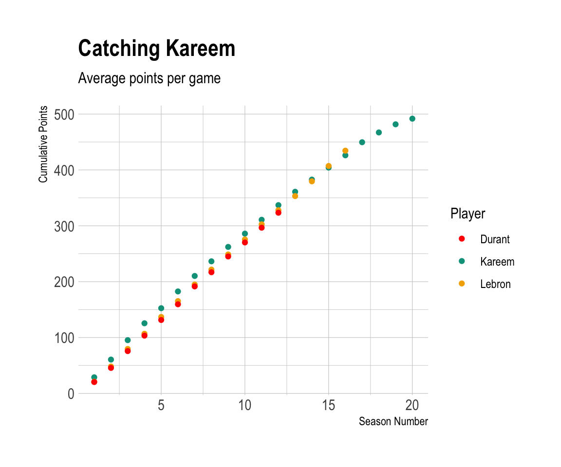
In Lebron’s most recent season, it looks like he finally caught Kareem. Did he?
tidied_clean %>%
  filter(season_num == 15) %>%
knitr::kable()| Season | player | season_num | season_points | cumulative_points |
|---|---|---|---|---|
| 1983-84 | Kareem | 15 | 21.5 | 404.2 |
| 2017-18 | Lebron | 15 | 27.5 | 407.1 |
Going by average points scored per game, he’s already overtaken Kareem. Swish.