98% green spaghetti, sliced and chopped
- 2018/15/04
- 18 min read
This is the latest stop in an analysis tour of free-range menu data.
One of the goals of fishing for real recipes is to be able to suss out patterns in how foods are combined and in what amounts in order to be able to generate new recipes. However, this post will mostly eschew creating anything useful and just mess around with the words in recipes themselves.
As a step toward creating new ingredients and recipes in interesting ways, we’ll
tag ingredient words with their parts of speech to find the most common noun-adjective pairs, and
create some menu mad libs.
For a sneak peek, here are a few that were created while I was putting this together.
| ingredient |
|---|
| 1/8 small, black round oil leaves - extract into cups |
| 3 cherry ribs, fully lime |
| 1 olive boneless, broken |
| 1/2 extra Sour carrots, lime for fluid pieces |
| 1/3 frozen onion, virgin |
| 1 Beef oil |
| 6 orange Mashed fresh Ranch |
| 1 Lindsay® |
So that deliciousness is what we have to look forward to at the end of this little experiment. Yummo.
Bit of Background
Up to this point we’ve scraped recipes from Allrecipes.com and tidied the resulting data, extracted ingredient unit names, and matched them their corresponding portion_abbreviations. We also munged the free text numbers into usable portion amounts (multiplying and averaging units where necessary to create) and converted these units into grams.
A glance at what the result of that looks like:
set.seed(123)

recipes_df %>%
  sample_n(10) %>%
  select(recipe_name, ingredients, portion_abbrev, portion, converted) %>%
  map_dfc(replace_na, "") %>%
kable()| recipe_name | ingredients | portion_abbrev | portion | converted |
|---|---|---|---|---|
| African Chicken in Spicy Red Sauce | 1 1/2 cups chopped onion | cup | 1.5 | 354.88 |
| Homemade Seasoned Salt | 1/4 cup kosher salt | cup | 0.25 | 59.15 |
| Calico Rice | 2 tablespoons picante sauce or salsa | tbsp | 2 | 29.57 |
| Poached Beef Fillet Served with its Own Broth and Baby Winter Vegetables | 8 ounces oxtail or beef shin | oz | 8 | 226.8 |
| Easy Puebla-Style Chicken Mole | 3 cups fat-free, low-sodium chicken broth | cup | 3 | 709.76 |
| Pork Picante | 1/4 teaspoon cayenne pepper | tsp | 0.25 | 1.23 |
| Candy Cane Cookies from Gold Medal® Flour | 2 large egg yolks | 2 | ||
| Chocolate-Raspberry Muffins | 1 1/2 teaspoons baking powder | tsp | 1.5 | 7.39 |
| Bhindi Masala (Spicy Okra Curry) | 1 teaspoon salt | tsp | 1 | 4.93 |
| Spaghetti and Meatballs (Paleo Style) | 1/2 cup cooked quinoa | cup | 0.5 | 118.29 |
Tagging Parts of Speech
In order to be able to combine ingredients in ways that might make sense, it’ll be useful to know the parts of speech of each word that makes up a given ingredient. The goal now is going to be to tag each word with its part of speech while retaining our tidy data format.
I’ll use the RDRPOSTagger package (beware, it does depend on rJava which can be a pain to install) to assign a part of speech (POS) to every word in every recipe.
First we define a model to use as our POS tagger.
library(RDRPOSTagger)
tagger <- rdr_model(language = "English", annotation = "POS")
Let’s see how the main rdr_pos() function works by tagging a few ingredients. The first argument is the model, which for us is tagger.
tagger %>%
  rdr_pos(recipes_df$ingredients[1:3]) %>%
  as_tibble() %>%
kable()| doc_id | token_id | token | pos |
|---|---|---|---|
| d1 | 1 | 1 | CD |
| d1 | 2 | (12 | CD |
| d1 | 3 | inch) | NN |
| d1 | 4 | pre | NN |
| d1 | 5 | - | : |
| d1 | 6 | baked | JJ |
| d1 | 7 | pizza | NN |
| d1 | 8 | crust | NN |
| d2 | 1 | 1 | CD |
| d2 | 2 | 1/2 | CD |
| d2 | 3 | cups | NNS |
| d2 | 4 | shredded | JJ |
| d2 | 5 | mozzarella | NNP |
| d2 | 6 | cheese | NN |
| d3 | 1 | 1 | CD |
| d3 | 2 | (14 | CD |
| d3 | 3 | ounce) | NN |
| d3 | 4 | jar | NN |
| d3 | 5 | pizza | NN |
| d3 | 6 | sauce | NN |
The pos column shows the acronym for the token’s part of speech.
A POS acronym-to-description key is below1:
| Tag | Description |
|---|---|
| CC | Coordinating conjunction |
| CD | Cardinal number |
| DT | Determiner |
| EX | Existential there |
| FW | Foreign word |
| IN | Preposition or subordinating conjunction |
| JJ | Adjective |
| JJR | Adjective, comparative |
| JJS | Adjective, superlative |
| LS | List item marker |
| MD | Modal |
| NN | Noun, singular or mass |
| NNS | Noun, plural |
| NNP | Proper noun, singular |
| NNPS | Proper noun, plural |
| PDT | Predeterminer |
| POS | Possessive ending |
| PRP | Personal pronoun |
| PRP$ | Possessive pronoun |
| RB | Adverb |
| RBR | Adverb, comparative |
| RBS | Adverb, superlative |
| RP | Particle |
| SYM | Symbol |
| TO | to |
| UH | Interjection |
| VB | Verb, base form |
| VBD | Verb, past tense |
| VBG | Verb, gerund or present participle |
| VBN | Verb, past participle |
| VBP | Verb, non-3rd person singular present |
| VBZ | Verb, 3rd person singular present |
| WDT | Wh-determiner |
| WP | Wh-pronoun |
| WP$ | Possessive wh-pronoun |
| WRB | Wh-adverb |
Modifying the Tagging Function
The rdr_pos() function gets us most of the way there, but I’ll make a slight adjustment to it in order to preserve more explicitly the relationship between the input and output.
By default, rdr_pos() names each doc_id as the default paste("d", seq_along(x), sep = "") where x is the input vector. That’s how we get d1, d2, etc. Instead of this default, we can ask this function to act more like a mutate by setting doc_id equal to our input’s recipe name concatenated with its ingredient. Then we only need to do a separate() on the <break> to dislodge our recipe name from its ingredient column. This explicitly relates input to output.
We’ll also want to include the rest of our original dataframe in the output. To keep things more compact, we nest() our POS tags into a data column so that we have one row per input before left_join()ing on our original dataframe.
recipe_sample <- recipes_df %>%
  slice(1:5)

tagged_sample <- tagger %>%
  RDRPOSTagger::rdr_pos(recipe_sample$ingredients,
          doc_id = paste(recipe_sample$recipe_name,
                         recipe_sample$ingredients,
                         sep = "<break>")) %>%
  separate(doc_id, into = c("recipe_name", "ingredients"), sep = "<break>") %>%
  nest(-recipe_name, -ingredients) %>%
  left_join(recipe_sample)
The result is easily unnested. I’ll show just a few columns here for space’s sake.
tagged_sample %>%
  unnest() %>%
  slice(1:5) %>%
  select(recipe_name, ingredients, token, pos, portion) %>%
kable()| recipe_name | ingredients | token | pos | portion |
|---|---|---|---|---|
| Johnsonville® Three Cheese Italian Style Chicken Sausage Skillet Pizza | 1 (12 inch) pre-baked pizza crust | 1 | CD | 12 |
| Johnsonville® Three Cheese Italian Style Chicken Sausage Skillet Pizza | 1 (12 inch) pre-baked pizza crust | (12 | CD | 12 |
| Johnsonville® Three Cheese Italian Style Chicken Sausage Skillet Pizza | 1 (12 inch) pre-baked pizza crust | inch) | NN | 12 |
| Johnsonville® Three Cheese Italian Style Chicken Sausage Skillet Pizza | 1 (12 inch) pre-baked pizza crust | pre | NN | 12 |
| Johnsonville® Three Cheese Italian Style Chicken Sausage Skillet Pizza | 1 (12 inch) pre-baked pizza crust | - | : | 12 |
It’s worth noting that some punctuation (like commas and periods) gets tagged as is, and some (like dashes and semicolons) gets a POS of ":". I’m not totally sure what the logic is behind that is, but it means that dashes, semicolons, and colons are treated interchangeably, whereas commas and periods are their own unique POS.
tagger %>%
  rdr_pos("foo , . - ; bar") %>%
kable()| doc_id | token_id | token | pos |
|---|---|---|---|
| d1 | 1 | foo | NN |
| d1 | 2 | , | , |
| d1 | 3 | . | . |
| d1 | 4 | - | : |
| d1 | 5 | ; | : |
| d1 | 6 | bar | NN |
If the distinction between dashes and semicolons is important, then when making mad libs we may down the line want to and only sub in punctuation marks for ones that are lexically equivalent.
Tagging a Dataframe
Let’s throw that bit of work into a function.
In tag_df() we’ll also get rid of all parentheses that often surround digits in order to be able to combine them with other words without any stray open or closed parentheses cluttering things up.
tag_df <- function(df, model = tagger) {

  df <- df %>%
    mutate(
      ingredients = ingredients %>% map_chr(str_replace_all, "[\\(\\)]", "")
    )

  inp <- df$ingredients

  tagged <- model %>%
     rdr_pos(inp,
          doc_id = glue::glue("{df$recipe_name}<break>{df$ingredients}")) %>%
    separate(doc_id,
             into = c("recipe_name", "ingredients"),
             sep = "<break>") %>%
    nest(-recipe_name, -ingredients) %>%
    left_join(df) %>%
    unnest()

  return(tagged)
}
And now we can tag our dataframe.
tagged_recipes_df <- recipes_df %>%
  tag_df()
What unique parts of speech do we have?
tibble("Tag" = unique(tagged_recipes_df$pos)) %>%
  left_join(pos_table, by = "Tag") %>%
kable()| Tag | Description |
|---|---|
| CD | Cardinal number |
| NN | Noun, singular or mass |
| : | NA |
| JJ | Adjective |
| NNS | Noun, plural |
| NNP | Proper noun, singular |
| , | NA |
| . | NA |
| VBN | Verb, past participle |
| VB | Verb, base form |
| CC | Coordinating conjunction |
| MD | Modal |
| VBZ | Verb, 3rd person singular present |
| IN | Preposition or subordinating conjunction |
| JJR | Adjective, comparative |
| RB | Adverb |
| TO | to |
| VBG | Verb, gerund or present participle |
| DT | Determiner |
| VBD | Verb, past tense |
| NNPS | Proper noun, plural |
| VBP | Verb, non-3rd person singular present |
| ’’ | NA |
| JJS | Adjective, superlative |
| RBR | Adverb, comparative |
| PRP$ | Possessive pronoun |
| SYM | Symbol |
| RP | Particle |
Common Consecutive Word Pairs
Now that we have each word’s part of speech, so now let’s see how words within ingredients relate to one another.
If we take a dplyr::lag() of our tagged dataframe, we can see the relationship between words that come directly after one another. token comes first, and token_lag second.
We can read the token_lag and token columns left to right now to see each pair of words in the sequence they appear in in the recipe.
tagged_recipes_df %>%
  group_by(recipe_name, ingredients) %>%
    mutate(
      token_id_lag = lag(token_id),
      token_lag = lag(token),
      pos_lag = lag(pos)
    ) %>%
  ungroup() %>%
  select(ingredients, token_lag, token, pos_lag, pos) %>%
  map_df(replace_na, "") %>%
  ungroup() %>%
  slice(1:5) %>%
kable()| ingredients | token_lag | token | pos_lag | pos |
|---|---|---|---|---|
| 1 12 inch pre-baked pizza crust | 1 | CD | ||
| 1 12 inch pre-baked pizza crust | 1 | 12 | CD | CD |
| 1 12 inch pre-baked pizza crust | 12 | inch | CD | NN |
| 1 12 inch pre-baked pizza crust | inch | pre | NN | NN |
| 1 12 inch pre-baked pizza crust | pre | - | NN | : |
We can throw this into a function that allows us to filter to any specific combination of token and token_lag parts of speech. By default we’ll set both to "NN" for nouns. (We use %in% in the filter() instead of == so that we can supply multiple possibilities for the parts of speech to keep.)
find_pos_pairs <- function(df, pos_lag_keep = 'NN', pos_keep = 'NN') {
  out <- df %>%
    group_by(recipe_name) %>%
    mutate(
      token_id_lag = lag(token_id),
      token_lag = lag(token),
      pos_lag = lag(pos)
    ) %>%
    select(
      ends_with("id"), ends_with("lag"), everything()
    ) %>%
    filter(pos %in% pos_keep & pos_lag %in% pos_lag_keep)

  return(out)
}
Using find_pos_pairs(), we can take untagged dataframe, tag it, and filter it a straightforward pipeline like this.
recipes_df %>%
  tag_df() %>%
  find_pos_pairs()
If our dataframe is already tagged, we can skip the tag_df() step, pass Go, and collect our POS pairs.
Let’s do that by looking at adjectives that precede nouns.
adj_noun_pos <- tagged_recipes_df %>%
  find_pos_pairs(pos_lag_keep = c("JJ", "JJR", "JJS"),         # All the adj types
                 pos_keep = c("NN", "NNS", "NNP", "NNPS"))  # All the noun types
Now a simple count of each distinct pair to see what the most common adj-noun combos are. These can be read left-to-right in the order they appear in ingredients.
adj_noun_pos_counts <- adj_noun_pos %>%
  group_by(token_lag, token) %>%
  count(sort = TRUE) %>%
  rename(n_pairs = n) %>%
  map_df(str_replace_all, "[\\()]", "")  # Remove parens

adj_noun_pos_counts %>%
  ungroup() %>%
  slice(1:15) %>%
kable()| token_lag | token | n_pairs |
|---|---|---|
| black | pepper | 76 |
| brown | sugar | 38 |
| white | sugar | 34 |
| garlic | powder | 22 |
| Cheddar | cheese | 21 |
| red | pepper | 20 |
| virgin | olive | 19 |
| sour | cream | 18 |
| green | onions | 17 |
| fluid | ounce | 16 |
| fresh | basil | 16 |
| lean | ground | 16 |
| green | bell | 15 |
| red | onion | 15 |
| fresh | cilantro | 13 |
From these counts we can draw up a quick scatterplot of the most frequent adjective-noun pairs in our recipes.
ggplot(adj_noun_pos_counts %>% ungroup() %>%
         top_n(15)) +
  geom_point(aes(reorder(token, n_pairs), reorder(token_lag, n_pairs),
                 size = n_pairs), stat = "identity") +
  ggtitle("Frequent Adjective-Noun Pairs") +
  labs(x = "Noun", y = "Adjective", size = "N Pairs") +
  theme_minimal(base_family = "Source Sans Pro") +
  theme(axis.text.x = element_text(angle = 45, hjust = 1))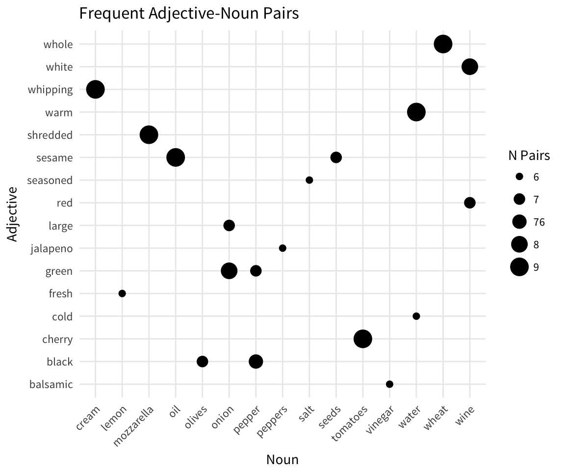
Menu Mad Libs
Now that we have every word tagged with its part of speech, we can mess around on the ingredient level.
Specifically, we’ll try swapping words with the same POS for one another to create a Frankenstein ingredient, mad lib style. In order to preserve the correct order of POS in an ingredient, we’ll use an existing ingredient as a template. The order of its parts of speech become the order of the POS in our mad lib.

Sampling Words
To start, let’s first sample a single ingredient from a single recipe.
set.seed(314159)

a_tagged_ingredient <-
  tagged_recipes_df %>%
  filter(recipe_name == sample(tagged_recipes_df$recipe_name, 1)) %>%
  filter(ingredients == sample(.$ingredients, 1)) %>%
  distinct(ingredients, recipe_name, token, pos)

a_tagged_ingredient %>%
  select(ingredients, token, pos) %>%
kable()| ingredients | token | pos |
|---|---|---|
| 2 cups crispy rice cereal such as Rice Krispies® | 2 | CD |
| 2 cups crispy rice cereal such as Rice Krispies® | cups | NNS |
| 2 cups crispy rice cereal such as Rice Krispies® | crispy | JJ |
| 2 cups crispy rice cereal such as Rice Krispies® | rice | NN |
| 2 cups crispy rice cereal such as Rice Krispies® | cereal | NN |
| 2 cups crispy rice cereal such as Rice Krispies® | such | JJ |
| 2 cups crispy rice cereal such as Rice Krispies® | as | IN |
| 2 cups crispy rice cereal such as Rice Krispies® | Rice | NNP |
| 2 cups crispy rice cereal such as Rice Krispies® | Krispies® | NNP |
Now for every word in our ingredient, we’ll use a mutate() to sample a new word with the same POS and relate it to the original word. The original word is in the token column, and its newly sampled counterpart is in the new_token column.
mad_libbed_ingredient <- a_tagged_ingredient %>%
  rowwise() %>%
  mutate(
    new_token = sample(tagged_recipes_df$token[which(tagged_recipes_df$pos == pos)], 1)
  ) %>%
  select(ingredients, token, new_token, pos)

mad_libbed_ingredient %>%
kable()| ingredients | token | new_token | pos |
|---|---|---|---|
| 2 cups crispy rice cereal such as Rice Krispies® | 2 | 1/2 | CD |
| 2 cups crispy rice cereal such as Rice Krispies® | cups | cups | NNS |
| 2 cups crispy rice cereal such as Rice Krispies® | crispy | softened | JJ |
| 2 cups crispy rice cereal such as Rice Krispies® | rice | butter | NN |
| 2 cups crispy rice cereal such as Rice Krispies® | cereal | Pinch | NN |
| 2 cups crispy rice cereal such as Rice Krispies® | such | sliced | JJ |
| 2 cups crispy rice cereal such as Rice Krispies® | as | of | IN |
| 2 cups crispy rice cereal such as Rice Krispies® | Rice | Chicken | NNP |
| 2 cups crispy rice cereal such as Rice Krispies® | Krispies® | KRAFT | NNP |
Cool so now we can read down the new_token column to get our mad libbed ingredient.
Let’s throw that all into a function called sample_token() which takes a part of speech to filter down to and a dataframe to sample from.
sample_token <- function(pos_want, population_df = tagged_recipes_df) {
  out_df <- population_df %>%
    ungroup() %>%
    filter(pos == pos_want)

  if (nrow(out_df) == 0) {
    out_token <- ""           # If we don't have any of that part of speech, return an empty string
  } else {
    out_token <- out_df %>%
      sample_n(1) %>%
      pull(token)
  }

  return(out_token)
}
Last step to complete our mad lib is to smush all the sampled tokens together into a single phrase. We concatenate everything with a space but at the very end do a pass through all commas, periods, semicolons, and colons to remove any leading spaces before them since (at least in English), we don’t don’t keep a space between preceding word and some punctuation.
collapse_tokens <- function(df) {
  df %>%
    pull(new_token) %>%
    str_c(collapse = " ") %>%
    str_replace_all("( [,\\.;:])", ",")
}
Now for each row in a dataframe, we can look at the POS in the token column, sample the same POS from our population dataframe (tagged_recipes_df by default), stick that in the same row in a new_token column, and finally collapse the new_token column down to a single ingredient.
a_tagged_ingredient %>%
  rowwise() %>%
  mutate(
    new_token = sample_token(pos)
  ) %>%
  collapse_tokens()
## [1] "1 sprigs garlic ounce ground whole into onion olive"Writing a Mad Lib
Putting sample_token() and collapse() into a function that returns a single mad lib. (The n_libs = 1 isn’t doing anything here at the moment since we’re only ever sampling one ingredient; we’ll get to it in a second.)
write_a_mad_lib <- function(n_libs = 1, col = ingredients, df = tagged_recipes_df) {

  q_col <- enquo(col)

  # Sample an ingredient template
  this_ing <- df %>%
    ungroup() %>%
    distinct(!!q_col) %>%
    sample_n(1) %>%
    pull(!!q_col)

  # Create new tokens from this template and collapse the new tokens into a mad lib
  this_lib <- df %>%
    filter(!!q_col == this_ing) %>%
    rowwise() %>%
    mutate(
    new_token = sample_token(pos) %>% replace_x()
    ) %>%
    collapse_tokens()

  return(this_lib)
}
Let’s take that function for a spin. Every time we run the function we’ll get a different mad lib, made from a different recipe template.
write_a_mad_lib()## [1] "1/4 cup Original or cream cracker"write_a_mad_lib()## [1] "1 sodium diced ounce peppers 3 soda yellow sauce cups 1 cup whole cup balls 115 ounce cored teaspoon raisins 2 turkey white sodium seeds"Now that we can write a single mad lib, what’s the best way to write many of them? A first approach could be to set up a for loop like so:
write_mad_libs_for <- function(n_libs = 5, df = tagged_recipes_df) {
  out <- vector(mode = "character", length = n_libs)

  for (i in seq(n_libs)) {
    this_ing <- df %>%
      ungroup() %>%
      distinct(ingredients) %>%
      sample_n(1) %>%
      pull(ingredients)

    this_lib <- df %>%
      filter(ingredients == this_ing) %>%
      rowwise() %>%
      mutate(
      new_token = sample_token(pos)
      ) %>%
      map_df(replace_na, "") %>%
      collapse_tokens()

    out[i] <- this_lib
  }

  return(out)
}write_mad_libs_for(3)## [1] "3 tablespoon all - inch garlic, and more as uncooked"
## [2] "1 oil thick ounce"
## [3] "2 packages crust - fresh fluid tablespoon, chopped and dried"Another approach would be to rewrite our original function, write_a_mad_lib(), to accept a vector. A third would be to pseudo-Vectorize write_a_mad_lib() so that we can map() over a number of arguments. (Thanks to Dean Attali’s post on Vectorize() for the inspiration here!)
I’m not super worried about performance, but let’s do the latter, just for fun. The argument we’ll vectorize is n_libs, which we had set to 1 by default in write_a_mad_lib.
write_mad_libs_vec <- Vectorize(write_a_mad_lib, vectorize.args = "n_libs")

1:3 %>% map_chr(write_mad_libs_vec)
## [1] "9 teaspoon drained green cup onion"
## [2] "17 water black tablespoons 1/4 teaspoon sliced peas"
## [3] "Swanson® chopped wide - ounce black butter"Let’s do a quick check to see how much our speed improved with Vectorize as compared to the for loop approach.
non_vectorized <- microbenchmark::microbenchmark(1 %>% write_mad_libs_for,
                                                 times = 100)
vectorized <- microbenchmark::microbenchmark(1 %>% write_mad_libs_vec,
                                             times = 100)

(time_ratio <- (median(vectorized$time) / median(non_vectorized$time)))
## [1] 1.050128So over 100 iterations, our vectorized function was on average about 5% faster than the for loop counterpart2.
Generating a bunch of Mad Libs
Now to write a bunch of mad libs!
set.seed(pi)

bunch_o_libs <- 1:50 %>%
  write_mad_libs_vec()

tibble(`Recipe Mad Libs` = bunch_o_libs) %>%
kable()| Recipe Mad Libs |
|---|
| 3 mixed free tablespoons, pitted and serve as filets |
| 2 water, freshly fluid |
| 4 teaspoon chopped dry Johnsonville |
| 1/2 walnuts sugar |
| 3/4 1 cumin cup parsley salsa sliced feta teaspoons |
| 2 beans juiced oil, pitted |
| 1 bittersweet salt |
| 1/4 white optional ounce chicken, curry in 1 1 - taste, garlic tablespoons |
| 3 2 tablespoons okra juice |
| 2 mayonnaise grated fluid thyme |
| loin and cheese |
| paprika or such ounce Onion or green soda |
| 1/3 teaspoons whole salt - small cinnamon cups |
| 3 sauce raisins, halved |
| 1/4 1 cups frozen white butter |
| 15 ounce garlic olive |
| 8 tub teaspoon |
| 1 cream Whipped cup chocolate |
| 1 1 cup pepper sliced - elbow substitute butter into heavy or anchovy |
| ounce Cheddar tablespoon to wine |
| 1 1 ounces Sweet diced ounce |
| 3/4 butter divided cream, unsweetened and beaten |
| 1 cup fresh ounce |
| 2 onion, divided or reduced |
| 1 peppers all - elbow Mexican |
| 1 garlic ground |
| 1 tomatoes large wheat sliced into Philadelphia Broccoli |
| 3 pork cored red vanilla |
| 1 2 teaspoon thick peas cayenne and vinegar |
| 6 cheese brown sprigs |
| ground olive cup cheese teaspoon |
| 1 broth fluid cup 12 teaspoon garlic cup 1 cup sweet cup |
| 2 spray warm artichoke |
| 1 pounds diced pound ground |
| 1 slices baking teaspoon, refrigerated |
| 3/4 teaspoons Shredded sugar walnut black of tomato BREAKSTONE’S |
| 3 cherry Seasoned cups, and to cup |
| 1 juice juice 1/2 syrup cup 2 salt pasta 1 breast oil 15 cup cup |
| 1 rice heavy soda |
| 2 marshmallows inch teaspoon |
| 1/3 2 Silver can grated ground, pitted |
| 1/4 1/4 tablespoons pepper |
| 1/4 butter virgin dried thighs |
| 6 broccoli shredded, peeled 1/2 Sugar cheddar, torn 2 basil LIGHT, grated |
| Guinness® |
| turkey to tablespoon ounce to teaspoon chocolate to cup pepper to oil chocolate to Peppermint cup to chicken |
| Organic avocado |
| 1/2 cup black teaspoon 1/2 style crosswise teaspoon 1 teaspoon balsamic celery 1 teaspoon dry cup 4 teaspoon garlic ounce 1 vegetable sliced fennel 1 pound couscous oil 2 teaspoon diced teaspoon |
| 1/4 inch teaspoon cloves |
| 1 fluid cranberries |
Sort of like real mad libs, most of these don’t make a lot of sense 😆. These make even less sense, partly because we’re replacing every word and not just certain words.
For a follow-up, we could work on improving them by weighting our sampling by the pairwise frequency of co-occurring words in our ingredients. If we build up ingredients that way, we should be more likely to sample a word that occurs more frequently in the context of the other words we have in our ingredient so far. While we’re at it, we could also generate mad-libbed recipe names in the same way (requires making tag_df() more flexible).
The mad libbed ingredients could also use a bit of general cleaning; we could take everything except brand names to lowercase and adjust whether a noun is singular or plural to match the context of the word preceding it (maybe using Bob Rudis’s great pluralize package). We might also consider treating units (e.g., “tablespoons” or “grams”) as a separate part of speech so they can’t be swapped in for regular nouns.
Hope you enjoyed this weird word scramble – till next time. 🍳
Source table was scraped and tidied into this dataframe.↩
That’s not as dramatic of a speedup as we would have gotten if we hadn’t reduced the amount of copies that need to be made at each iteration by allocating space in output vector jumping into the loop (using
out <- vector(mode = "character", length = n_libs)).↩