Monkeys are like Onions
- 2018/25/03
- 14 min read
This is part two of a series on scraping content from the satirical news site The Onion and feeding that content to the newly-spruced up monkeylearn package. Part one deals with the scraping and munging of the data itself. In this chunk of work, we’ll go about classifying that data and getting a very unscientific measure of how “well” the classifier performed1.
MonkeyLearn Background
I’ve spent a really fun chunk of time in the last month or so developing the rOpenSci package text processing package monkeylearn along with the fantastic research software engineer Maëlle Salmon. The package is an R interface to the MonkeyLearn API, which is a cloud platform for text classification and keyword extraction. The service allows you to train your own classifier or use one of their pre-trained extraction or classification “modules.” Those modules are specialized to classify or extract certain information from text. The type of results they return depend on the classifier or extractor the user supplies.
I use the package in my work at Earlybird, which is the reason I originally first started contributing to it, but wanted to test it out on some more fun data. Since there is a pre-trained “News” classifier available from MonkeyLearn, I was interested in how that classifier would handle satirical news from the humor site The Onion.
Refresher
library(dobtools)    # devtools::install_github("aedobbyn/dobtools")
library(tidyverse)
library(stringr)
library(monkeylearn)
library(rvest)
In part one, we defined our subdomains
subdomains <- c("www", "politics", "local", "sports", "entertainment", "opinion")and saved our freshly-rvested texts in an object all_texts_clean. We’ll use that as our jumping-off point here.
I’ll use our same trim_content helper from before to be able to show a manageable amount of a dataframe with a lot of text in kable format. By default it samples three rows and takes just the first 50 characters of a given column supplied (here, the column content).
dobtools::trim_content## function (df, col = content, last_char = 50, sample_some = 3)
## {
## assertthat::assert_that(deparse(substitute(col)) %in% names(df),
## msg = "col supplied must be present in df")
## assertthat::assert_that(is.null(sample_some) || is.numeric(sample_some),
## msg = "sample_some must be NULL or numeric")
## if (!is.null(sample_some)) {
## df <- df %>% dplyr::sample_n(sample_some)
## }
## q_col <- rlang::enquo(col)
## out <- df %>% dplyr::rowwise() %>% dplyr::mutate_at(dplyr::vars(!(!q_col)),
## substr, 1, last_char)
## return(out)
## }
## <environment: namespace:dobtools>all_texts_clean %>%
trim_content() %>%
kable()| content | subd | link | referring_url | referring_subd |
|---|---|---|---|---|
| NEW YORK—Saying that he was able to draw upon a li | local | https://local.theonion.com/classically-trained-actor-can-talk-on-cue-1823995491 | https://local.theonion.com | local |
| NEW YORK—Shifting creative gears to pursue what he | entertainment | https://entertainment.theonion.com/paul-giamatti-cuts-back-on-acting-to-focus-on-signature-1823828872 | https://entertainment.theonion.com | entertainment |
| LOS GATOS, CA—Acknowledging that the former presid | entertainment | https://entertainment.theonion.com/netflix-executive-unsure-how-to-tell-barack-obama-his-s-1823651466 | https://entertainment.theonion.com | entertainment |
Today I [Monkey]Learned
We can peruse the pretrained MonkeyLearn modules (keyword extractors and text classifiers) at https://app.monkeylearn.com/main/explore/ or use monkeylearn::monkeylearn_classifiers() to get a list of pre-trained classifiers and their descriptions.
A sample:
monkeylearn_classifiers() %>%
  select(classifier_id, name, description) %>%
  sample_n(5) %>%
kable()| classifier_id | name | description |
|---|---|---|
| cl_mcHq5Mxu | Generic Sentiment | Classify texts in English according to their sentiment: positive, neutral or negative. |
| cl_u9PRHNzf | Tweets Sentiment (Spanish) | Classifying tweets in Spanish (from Spain) according to their sentiment: positive, neutral or negative. |
| cl_hT2jYBHR | Ofertas de trabajo | Classifies job postings in Spanish according to its topic. |
| cl_rtdVEb8p | Telcos - Sentiment analysis (Facebook) | Classify Facebook posts and comments in Telcos pages according to its sentiment. |
| cl_uEzzFRHh | Telcos - Needs Help Detection (Facebook) | Classify Facebook posts and comments in Telcos pages to detect if a user needs help from a customer support representative or not. |
The two classifiers that look the most promising are the News classifier (ID cl_hS9wMk9y) and the Events classifier (ID cl_4omNGduL).
monkeylearn_classifiers() %>%
  select(classifier_id, name, description) %>%
  filter(name %in% c("Events Classifier", "News Classifier")) %>%
kable()| classifier_id | name | description |
|---|---|---|
| cl_4omNGduL | Events Classifier | Classify events according to their description. |
| cl_hS9wMk9y | News Classifier | Classify news by topics like Sports, Politics, Business and more. |
![]()
First we’ll test the News one on a sample text.
text_sample <- all_texts_clean %>%
  sample_n(1)
Let’s take a look at this link’s content.
text_sample %>%
  select(content) %>%
kable()| content |
|---|
| NEW YORK—Shifting creative gears to pursue what he called “his other great passion in life,” casual men’s fashion, Paul Giamatti announced Friday that he would be cutting back on acting to launch a signature line of shapeless khakis and rumpled polos. “Over the years, I’ve heard from so many fans who wanted to dress like my characters that I figured, why not? I’ll try designing loose-fitting, haphazard looks that evoke the classic ‘Giamatti’ brand,” the 50-year-old Brooklyn native told fashion reporters, confirming that his not-quite-ready-to-wear line would range in size from large to extra large and be sold exclusively at Kohl’s. “We’re also featuring faded golf hats, shabby corduroy sport coats, loafers, and unnecessarily long button-downs. And if you were wondering how the pants are cut, don’t worry—there will be ample roominess around the crotch.” The official release of the Giamatti line will occur later this month with a runway show whenever East Windsor, New Jersey’s historic Bowling & Recreation Center can fit it in. |
Cool. Now a bit on the monkey_ functions (which you can see more examples of in the vignette).
The monkey_classify() fuction takes either a vector of texts or a dataframe and a named column. It’ll always return a dataframe relating your input to your output. You can set the number of texts you want batched to the API (up to 200) with the texts_per_req parameter. (This is much, much faster than going one-by-one.) Here we’ve got only a single text, so we’ll have just one batch. What does our output look like?
text_sample %>%
  monkey_classify(col = content, classifier_id = "cl_hS9wMk9y") %>%
  trim_content(sample_some = 2) %>%
  kable()
## Processing batch 1 of 1 batches: texts 1 to 1| content | category_id | probability | label |
|---|---|---|---|
| NEW YORK—Shifting creative gears to pursue what he | 53873822 | 0.268 | Fashion & Style |
| NEW YORK—Shifting creative gears to pursue what he | 53873812 | 0.403 | Living |
We get multiple classificationlabels for each input content, along with a unique category_id and probability. For now, we only really care about the label.
Scaling Up
Let’s run the News and Events classifiers on all_texts_clean. The .keep_all option allows us to retain all columns from the input dataframe, so that monkey_classify() acts like a mutate, tacking on a new result column to our input. If set to FALSE, it would return only the input col and its corresponding output res.
all_texts_classified_news_nested <- all_texts_clean %>%
  monkey_classify(
    col = content,
    classifier_id = "cl_hS9wMk9y"
    unnest = FALSE,
    .keep_all = TRUE,
    verbose = FALSE)

all_texts_classified_events_nested <- all_texts_clean %>%
  monkey_classify(
    col = content,
    classifier_id = "cl_4omNGduL",
    unnest = FALSE,
    .keep_all = TRUE,
    verbose = FALSE)
I set unnest to FALSE in order to be able to check that the two classifiers returned data of the same dimensions. Each should have one row per input, even if there are 0 or multiple classifications for that input.
assertthat::are_equal(dim(all_texts_classified_news_nested),
                      dim(all_texts_classified_events_nested))
## [1] TRUETaking a look at just the output of the News classifier, we see we have a nested list-col called res, the result of our round-trip to MonkeyLearn.
(news_samp <- all_texts_classified_news_nested %>%
  trim_content() %>%
   select(content, res, everything()))
## Source: local data frame [3 x 6]
## Groups: <by row>
##
## # A tibble: 3 x 6
## content res subd link referring_url referring_subd
## <chr> <list> <chr> <chr> <chr> <chr>
## 1 LOS ANGELES… <data.… ente… https://enter… https://entert… entertainment
## 2 BURBANK, CA… <data.… ente… https://enter… https://entert… entertainment
## 3 WASHINGTON—… <data.… poli… https://polit… https://politi… politicsIf we unnest res, we’ll be able to see all our labels as we did in our text_sample above.
news_samp %>%
  unnest() %>%
  select(content, label, category_id, probability, everything()) %>%
kable()Now we’ll join our News and Events results on the common column, content to end up with a label_news and label_events column for each input.
classified <- all_texts_classified_news_nested %>% unnest() %>%
  left_join(all_texts_classified_events_nested %>% unnest(), by = "content")

names(classified) <- names(classified) %>%
  str_replace_all("\\.x", "_news") %>%
  str_replace_all("\\.y", "_events")
After a bit of cleaning up, we’re left with a dataframe, classified, relating each input to its News and Events classifications along with its subdomain and information about the link that pointed us to that article.
(classified <- classified %>%
  rename(link = link_news,
         subd = subd_news,
         referring_url = referring_url_news,
         referring_subd = referring_subd_news) %>%
  select(subd, content, link, label_news, label_events,
         referring_url, referring_subd,
         probability_news, probability_events))
## # A tibble: 220 x 9
## subd content link label_news label_events referring_url
## <chr> <chr> <chr> <chr> <chr> <chr>
## 1 polit… WASHINGTON—In an ef… http… Science &… Entertainme… https://poli…
## 2 polit… WASHINGTON—In an ef… http… Science &… Sports https://poli…
## 3 polit… WASHINGTON—In an ef… http… Science &… Soccer https://poli…
## 4 polit… WASHINGTON—In an ef… http… Energy & … Entertainme… https://poli…
## 5 polit… WASHINGTON—In an ef… http… Energy & … Sports https://poli…
## 6 polit… WASHINGTON—In an ef… http… Energy & … Soccer https://poli…
## 7 polit… WASHINGTON—In the l… http… Arts & Cu… Entertainme… https://poli…
## 8 polit… WASHINGTON—In the l… http… Arts & Cu… Sports https://poli…
## 9 polit… WASHINGTON—In the l… http… Arts & Cu… Fighting & … https://poli…
## 10 polit… WASHINGTON—In the l… http… TV & Radio Entertainme… https://poli…
## # ... with 210 more rows, and 3 more variables: referring_subd <chr>,
## # probability_news <dbl>, probability_events <dbl>To show a sample:
classified %>%
  trim_content() %>%
kable()| subd | content | link | label_news | label_events | referring_url | referring_subd | probability_news | probability_events |
|---|---|---|---|---|---|---|---|---|
| entertainment | NEW YORK—Shifting creative gears to pursue what he | https://entertainment.theonion.com/paul-giamatti-cuts-back-on-acting-to-focus-on-signature-1823828872 | Fashion & Style | Beauty & Fashion | https://entertainment.theonion.com | entertainment | 0.268 | 0.272 |
| politics | WASHINGTON—In an effort to guarantee Americans the | https://politics.theonion.com/epa-rolls-back-emissions-standards-to-increase-consumer-1824218100 | Energy & Environment | Soccer | https://politics.theonion.com | politics | 0.406 | 0.102 |
| local | JUNEAU, AK—Saying it was clear the parents never i | https://local.theonion.com/family-has-way-too-many-daughters-for-them-not-to-have-1824313914 | World | Soccer | https://local.theonion.com | local | 0.211 | 0.114 |
Evaluate
Now we can ask how accurate our MonkeyLearn classifications were. For instance, how often are texts that appear under the politics subdomain tagged with the Politics label?
What are the possible classifications for our News classifier?
(news_labels <- classified$label_news %>% unique())## [1] "Science & Technology" "Energy & Environment"
## [3] "Arts & Culture" "TV & Radio"
## [5] "World" "Asia & Pacific"
## [7] "Music" "U.S."
## [9] "Living" "Fashion & Style"
## [11] "Books" "Business"
## [13] "Companies" "Family & Relationships"
## [15] "Home" "Food"
## [17] "Career" "Sports"
## [19] "Baseball" "Football"
## [21] "Basketball" "Movies"And Events?
(events_labels <- classified$label_events %>% unique())## [1] "Entertainment" "Sports"
## [3] "Soccer" "Fighting & Martial Arts"
## [5] "Movements & Ideologies" "Politics"
## [7] "Arts & Culture" "Music"
## [9] "Charity & Non-Profits" "Football"
## [11] "Family & Children" "Food & Drink"
## [13] "Baseball" "Beauty & Fashion"
## [15] "Film" "Dance & Theatre"Now we have to square these labels with our subdomains, i.e., www, politics, local, sports, entertainment, opinion, in order to be able to evaluate how well the classifications matched up.
We’ll collapse certain classifications into others and remove some that we can’t clearly align with one or another subdomain.
Of course all of this is purely subjective; you could easily argue that “Food” belongs in entertainment rather than local and of course there’s no way for us to know whether, for example, articles published at the sports subdomain really are always about sports.
entertainment <-
  c("Entertainment",
          "Arts & Culture", "Books", "Film", "Music", "TV & Radio")
local <-
  c("Local",
          "Food", "Living")
politics <-
  c("Politics",
          "Middle East", "Movements & Ideologies", "U.S.", "World")
sports <-
  c("Sports",
          "Baseball", "Cycling", "Football", "Soccer")
![]()
Now we’ll create a dplyr::case_when() switch statement inside a mutate() to assign a collapsed_label column.
classified_relabeled <- classified %>%
  drop_na(label_news, label_events) %>%
  rowwise() %>%
  mutate(
    collapsed_label = case_when(
      label_news %in% entertainment || label_events %in% entertainment ~ "entertainment",
      label_news %in% local || label_events %in% local ~ "local",
      label_news %in% politics || label_events %in% politics ~ "politics",
      label_news %in% sports || label_events %in% sports ~ "sports"
    )
  ) %>%
  replace_na(list(collapsed_label = "www")) %>%   # If none of the above, we give it www
  select(subd, collapsed_label, content, everything())

classified_relabeled$collapsed_label <- as.character(classified_relabeled$collapsed_label)
We drop rows that weren’t classified with any of the entertainment, local, politics, or sports classifiers and then determine whether the MonkeyLearn classification lined up with the Onion subdomain.
If the MonkeyLearn label is the same as the subdomain we give match a TRUE, and a FALSE otherwise.
classified_relabeled_confusion <-
  classified_relabeled %>%
  select(subd, collapsed_label) %>%
  drop_na(collapsed_label) %>%
  rowwise() %>%
  mutate(
    match = case_when(
      identical(collapsed_label, subd) ~ TRUE,
      !(identical(collapsed_label, subd)) ~ FALSE
    )
  )
Now we can calculate how “well” the classifier did. First, our overall accuracy compared to chance:
n_subs <- length(levels(factor(classified_relabeled$collapsed_label)))

overall_accuracy <- classified_relabeled_confusion %>%
  ungroup() %>%
  summarise(
    overall_accuracy = sum(match == TRUE) / nrow(.),
    chance = 1 / n_subs
  )

overall_accuracy %>% kable()| overall_accuracy | chance |
|---|---|
| 0.4272727 | 0.2 |
Next, we can break this down by subdomain.
accuracy_per_subd <- classified_relabeled_confusion %>%
  ungroup() %>%
  group_by(subd) %>%
  add_count() %>%
  rename(n_total = n) %>%
  group_by(collapsed_label, subd) %>%
  add_count(sort = TRUE) %>%
  rename(n_correct = n) %>%
  ungroup() %>%
  distinct(subd, collapsed_label, n_total, n_correct, match) %>%
  arrange(subd, desc(n_total), desc(n_correct))


accuracy_per_subd %>% kable()| subd | collapsed_label | match | n_total | n_correct |
|---|---|---|---|---|
| entertainment | entertainment | TRUE | 58 | 44 |
| entertainment | politics | FALSE | 58 | 4 |
| entertainment | sports | FALSE | 58 | 4 |
| entertainment | local | FALSE | 58 | 3 |
| entertainment | www | FALSE | 58 | 3 |
| local | entertainment | FALSE | 62 | 34 |
| local | local | TRUE | 62 | 12 |
| local | sports | FALSE | 62 | 10 |
| local | politics | FALSE | 62 | 4 |
| local | www | FALSE | 62 | 2 |
| politics | entertainment | FALSE | 76 | 40 |
| politics | politics | TRUE | 76 | 22 |
| politics | sports | FALSE | 76 | 12 |
| politics | local | FALSE | 76 | 2 |
| sports | sports | TRUE | 24 | 16 |
| sports | entertainment | FALSE | 24 | 8 |
Let’s find our percent correct for each subdomain by taking just the matches and seeing how many “correct” matches out of the total we had.
perc_correct <- accuracy_per_subd %>%
  filter(match == TRUE) %>%
  mutate(
    perc = n_correct / n_total
  )

perc_correct %>% kable()| subd | collapsed_label | match | n_total | n_correct | perc |
|---|---|---|---|---|---|
| entertainment | entertainment | TRUE | 58 | 44 | 0.7586207 |
| local | local | TRUE | 62 | 12 | 0.1935484 |
| politics | politics | TRUE | 76 | 22 | 0.2894737 |
| sports | sports | TRUE | 24 | 16 | 0.6666667 |
Now we can plot these percentages as compared to chance:
ggplot(perc_correct) +
  geom_bar(aes(collapsed_label %>% map_chr(dobtools::cap_it), perc),
           width = 0.5,
           stat = "identity",
           position = "dodge",
           colour = "#212529", fill = "white") +
  geom_hline(aes(yintercept = overall_accuracy$chance),
             linetype = "dotted") +
  ggtitle("The Onion articles, Correctly Classified") +
  labs(x = "Subdomain", y = "Percent Correctly MonkeyLearn Classified",
     subtitle = "Using the MonkeyLearn API") +
  theme_minimal(base_family = "Source Sans Pro")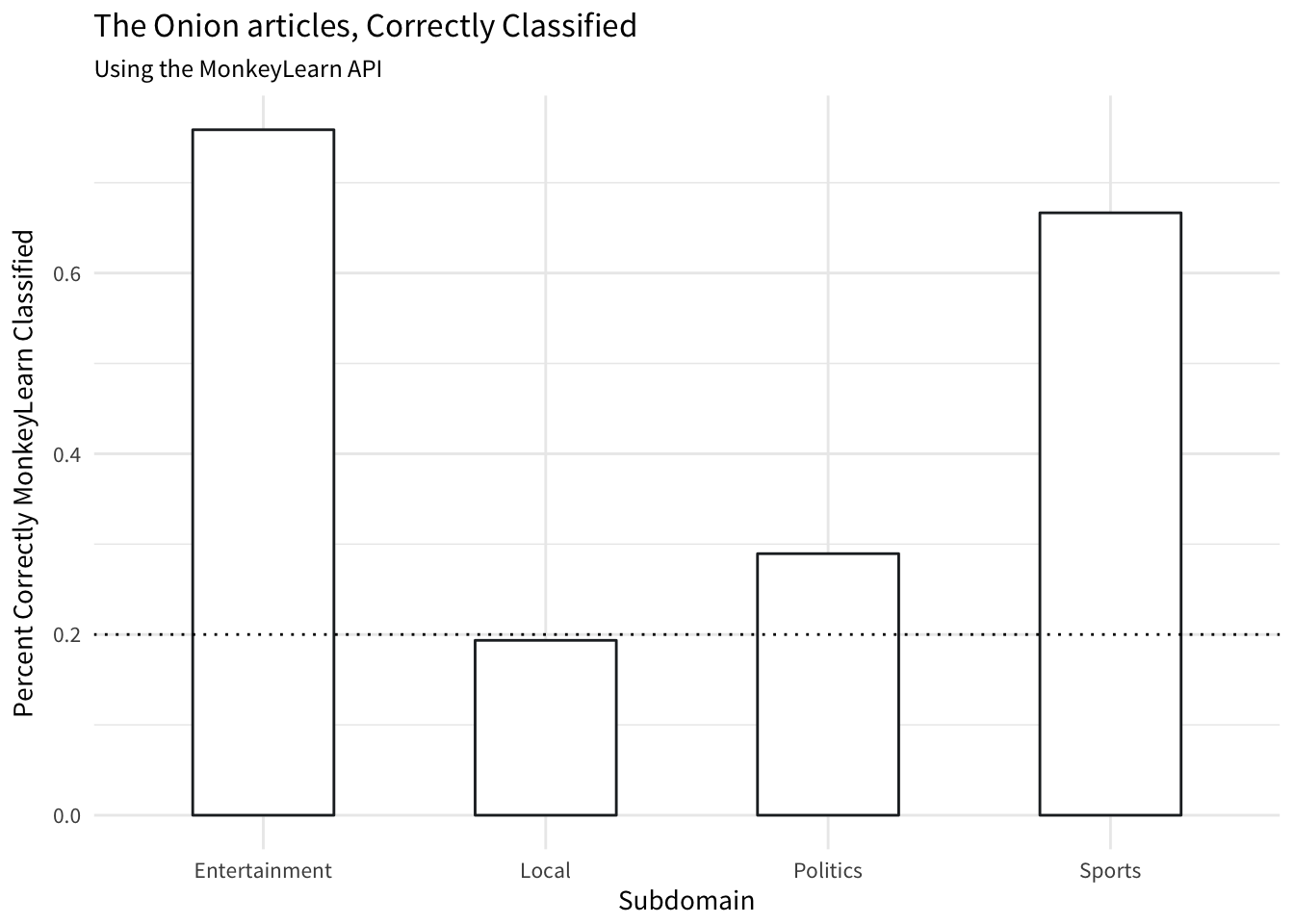
It make sense that Local articles have low accuracy as these were given the most amorphous tags of Local, Food, Living.
When MonkeyLearn went wrong, where did it go wrong?
We’ll plot the full spread, broken into quadrants by subdomain.
accuracy_per_subd %>%
  mutate(
    perc = n_correct / n_total
  ) %>%
  ggplot() +
  geom_bar(aes(collapsed_label %>%
                 map_chr(dobtools::cap_it), perc,
               colour = factor(match)),
           stat = "identity",
           width = 0.5,
           fill = "white") +
  geom_hline(aes(yintercept = overall_accuracy$chance),
             linetype = "dotted") +
  facet_wrap(~ subd %>% map_chr(dobtools::cap_it)) +
  scale_colour_manual(values = c("#27265f", "#e83e8c"), name = "A match?") +
  ggtitle("The Onion articles, Full Breakdown by Subdomain") +
  labs(x = "Classification", y = "Percent assigned this Classification",
     subtitle = "When incorrect, what classification were they assigned?",
     colour = "A match?", fill = "A match?") +
  theme_minimal(base_family = "Source Sans Pro") +
  theme(axis.text.x = element_text(angle = 45, hjust = 1))
The classifications are best for Sports and Entertainment articles, while entertainment is over-assigned to Local and Politics articles. Of course, our measure of segmenting MonkeyLearn classifications into subdomains was artificial from the get-go, so all of this is easily challengeable.
Closing Thoughts
In this toy example we can see that the MonkeyLearn API is flexible enough to classify texts it’s never seen before. Of course we’re not measuring its accuracy rigorously, but from our proxy for validating how well it was able to classify texts into the correct category we can show that it at least performed above chance. The monkeylearn package interface makes it trivial to feed in a dataframe of texts and receive a nicely formatted dataframe in return.
Future Directions
Thinking of next places to take this, we might consider examining the network relationships between referring subdomains and content subdomains, or doing a text analysis of the words in articles that tend crop up most frequently when classified with a certain label (as compared to how frequently they appear when assigned a different label). Another direction would be to train a fake news detector (using a MonkeyLearn module or rolling our own, maybe Naïve Bayes to start) on The Onion and real news articles of similar sizes.