On Brewing Beer-in-Hand Data Science

Backstory

It’s a typical Thursday around beer o’clock and a few coworkers and I are hanging out in the office. We’ve got some brews and whiteboard which, as my coworker Kris points out, is a failsafe great combination. I don’t pretend to be a beer aficionado, but Kris is the real deal; in addition to being an excellent web developer, Kris and his girlfriend man the popular Instagram account kmkbeer. Around this time, Kris had started building an app for rating beers on a variety of dimensions, so you could rate, say, Deschutes’s Fresh Squeezed IPA on maltiness, sweetness and a host of other dimensions. That way you could remember not just that it’s a 4.5/5 stars but that it’s pretty juicy, all things considered.

The main sticking point – and this is where the whiteboard markers came out – is that you’d want to be able to capture that a beer tasted smoky for a porter or was hoppy for a wheat beer. That’s important because a very hoppy wheat beer might be considred quite a mildly hopped IPA. At this point we started drawing some distribution density curves and thinking about setting priors for every style. That prior would be the flavor baseline for each type of beer, allowing you to make these types of “for a” distinctions on the style level.

This is about when I started thinking about the concept of beer “styles” in general. You’ve got – at the highest split – your ales and your lagers, and then within those categories you’ve got pale ales and IPLs and kölschs and double IPAs and whatnot; that is, the categories people typically recognize as beer syles.

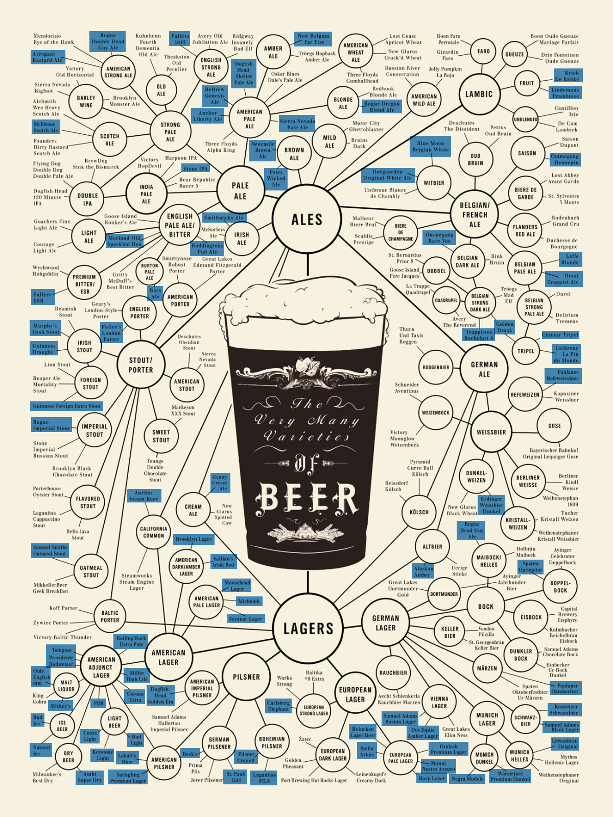
But: are styles even the best way of dividing up beers? Or is it just the easiest and most immediate heuristic we’ve got? Assuming that beers do necessarily fit well into styles is a bit circular; we only have the style paradigm to work off of, so if we’re tasked with classifying a beer we’re likely to reach for style as an easy way to bucket beers.

This brought me to thinking about clustering, of course. If styles do define the beer landscape well, then styles boundaries should more or less match up with cluster boundaries. If they don’t, well, that would be some evidence that the beer landscape is more of an overlapping mush than a few natrually neat, cut-and-dry buckets and that maybe some stouts are actually closer to porters than they are to the typical stout, or whatever the case may be.

So! Where to get the data, though. The usual question. Well, Kris mentioned an online database called BreweryDB, so, armed with a URL and a question I was interested in, I decided to check it out.

Getting Data

BreweryDB offers a RESTful API; if you’re not familiar, what that means is that once you’ve created an API key ¹, you can hand that key over in a URL with certain query parameters and receive data back. The documentation will tell you how what types of data are available and how you should structure your request to get the data you want. The one caveat in the BreweryDB case is you won’t get everything the API has to offer without creating a premium key ($6 a month); once you do, you’ll get unlimited requests and a few extra endpoints beyond what you get at the free tier.

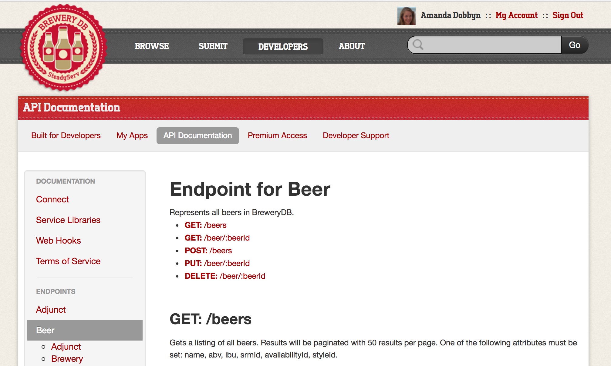
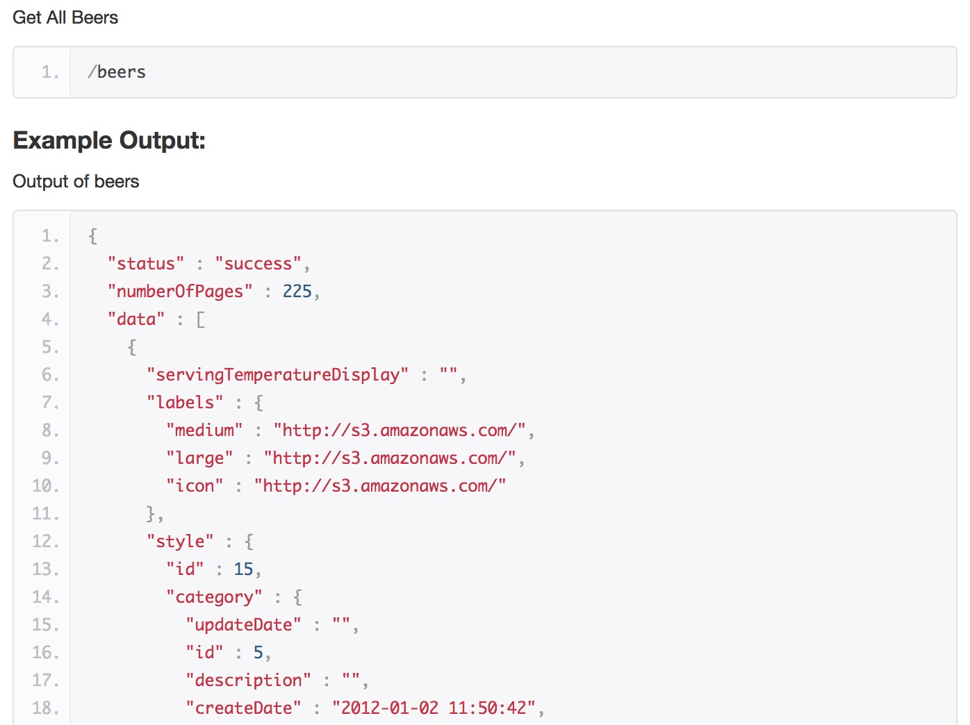
A look through the BreweryDB API documentation shows that we can get data back as JSON (the default), XML, or serialized PHP. We’ll be asking for JSON. If you’re requesting data on a single beer, you’d supply a URL that contains the endpoint beer, the beer’s ID, and your key like so: http://api.brewerydb.com/v2/beer/BEER_ID_HERE/?key=/YOUR_KEY_HERE.

If you entered such a URL in the browser, the response looks like:

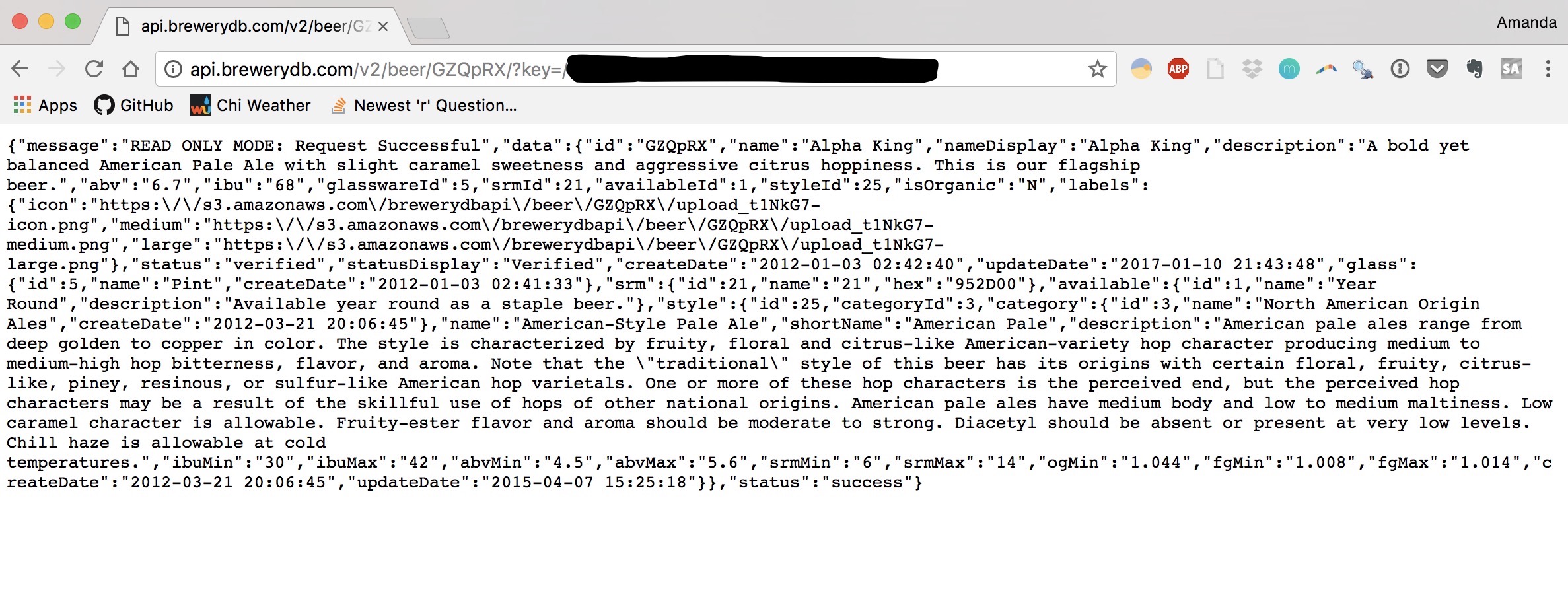
That’s beer data! But not that useful yet. We want to take that JSON and fit it into a tidy dataframe. To do that, I turned to the excellent jsonlite package, which has a few functions for converting from JSON to R objects (generally lists because they can be easily nested like JSON) and vice versa. The main function we’ll need is fromJSON(). Underneath jsonlite are the httr and curl packages that allows you to construct HTTP requests in a straightforward way; what fromJSON() in particular does is take a URL, write a GET request for you, and give you back the reponse as a nested list.

To get our feet wet, we can generalize the URL from above and write a little function that takes a beer ID and returns a nested list of data.

base_url <- "http://api.brewerydb.com/v2"
key_preface <- "/?key="

get_beer <- function(id) {
  jsonlite::fromJSON(paste0(base_url, "/beer/", id, "/", key_preface, key))
}

Okay so now we can request a given beer by its ID. I’ll spare you the entire output, but here’s the basic structure:

get_beer("GZQpRX") %>% str(list.len = 15)

## List of 3
##  $ message: chr "READ ONLY MODE: Request Successful"
##  $ data   :List of 20
##   ..$ id           : chr "GZQpRX"
##   ..$ name         : chr "Alpha King"
##   ..$ nameDisplay  : chr "Alpha King"
##   ..$ description  : chr "A bold yet balanced American Pale Ale with slight caramel sweetness and aggressive citrus hoppiness. This is our flagship beer."| __truncated__
##   ..$ abv          : chr "6.7"
##   ..$ ibu          : chr "68"
##   ..$ glasswareId  : int 5
##   ..$ srmId        : int 21
##   ..$ availableId  : int 1
##   ..$ styleId      : int 25
##   ..$ isOrganic    : chr "N"
##   ..$ labels       :List of 3
##   .. ..$ icon  : chr "https://s3.amazonaws.com/brewerydbapi/beer/GZQpRX/upload_t1NkG7-icon.png"
##   .. ..$ medium: chr "https://s3.amazonaws.com/brewerydbapi/beer/GZQpRX/upload_t1NkG7-medium.png"
##   .. ..$ large : chr "https://s3.amazonaws.com/brewerydbapi/beer/GZQpRX/upload_t1NkG7-large.png"
##   ..$ status       : chr "verified"
##   ..$ statusDisplay: chr "Verified"
##   ..$ createDate   : chr "2012-01-03 02:42:40"
##   .. [list output truncated]
##  $ status : chr "success"

and the first few elements

get_beer("GZQpRX")$data[1:5]

## $id
## [1] "GZQpRX"
## 
## $name
## [1] "Alpha King"
## 
## $nameDisplay
## [1] "Alpha King"
## 
## $description
## [1] "A bold yet balanced American Pale Ale with slight caramel sweetness and aggressive citrus hoppiness. This is our flagship beer."
## 
## $abv
## [1] "6.7"

 

If we wanted to go back to JSON we can take a list like that and, you guessed it, use toJSON():

get_beer("GZQpRX") %>% toJSON()

## {"message":["READ ONLY MODE: Request Successful"],"data":{"id":["GZQpRX"],"name":["Alpha King"],"nameDisplay":["Alpha King"],"description":["A bold yet balanced American Pale Ale with slight caramel sweetness and aggressive citrus hoppiness. This is our flagship beer."],"abv":["6.7"],"ibu":["68"],"glasswareId":[5],"srmId":[21],"availableId":[1],"styleId":[25],"isOrganic":["N"],"labels":{"icon":["https://s3.amazonaws.com/brewerydbapi/beer/GZQpRX/upload_t1NkG7-icon.png"],"medium":["https://s3.amazonaws.com/brewerydbapi/beer/GZQpRX/upload_t1NkG7-medium.png"],"large":["https://s3.amazonaws.com/brewerydbapi/beer/GZQpRX/upload_t1NkG7-large.png"]},"status":["verified"],"statusDisplay":["Verified"],"createDate":["2012-01-03 02:42:40"],"updateDate":["2017-01-10 21:43:48"],"glass":{"id":[5],"name":["Pint"],"createDate":["2012-01-03 02:41:33"]},"srm":{"id":[21],"name":["21"],"hex":["952D00"]},"available":{"id":[1],"name":["Year Round"],"description":["Available year round as a staple beer."]},"style":{"id":[25],"categoryId":[3],"category":{"id":[3],"name":["North American Origin Ales"],"createDate":["2012-03-21 20:06:45"]},"name":["American-Style Pale Ale"],"shortName":["American Pale"],"description":["American pale ales range from deep golden to copper in color. The style is characterized by fruity, floral and citrus-like American-variety hop character producing medium to medium-high hop bitterness, flavor, and aroma. Note that the \"traditional\" style of this beer has its origins with certain floral, fruity, citrus-like, piney, resinous, or sulfur-like American hop varietals. One or more of these hop characters is the perceived end, but the perceived hop characters may be a result of the skillful use of hops of other national origins. American pale ales have medium body and low to medium maltiness. Low caramel character is allowable. Fruity-ester flavor and aroma should be moderate to strong. Diacetyl should be absent or present at very low levels. Chill haze is allowable at cold temperatures."],"ibuMin":["30"],"ibuMax":["42"],"abvMin":["4.5"],"abvMax":["5.6"],"srmMin":["6"],"srmMax":["14"],"ogMin":["1.044"],"fgMin":["1.008"],"fgMax":["1.014"],"createDate":["2012-03-21 20:06:45"],"updateDate":["2015-04-07 15:25:18"]}},"status":["success"]}

 

BreweryDB’s got several endpoints that take a single parameter, an ID, just like the beer endpoint that we based our function on. I wanted a function for each of these endpoints so I could quickly take a look at the structure of the data returned. Rather than construct them all by hand like we did with get_beer(), this seemed like a good time to write a function factory to create functions to GET any beer, brewery, category, etc. if we know its ID.

First, a vector of all the single-parameter endpoints:

endpoints <- c("beer", "brewery", "category", "event", "feature", 
               "glass", "guild", "hop", "ingredient", "location", 
               "socialsite", "style", "menu")

Next we’ll write a generic function for getting data about a single ID, id from an endpoint ep.

# Base function
get_ <- function(id, ep) {
  jsonlite::fromJSON(paste0(base_url, "/", ep, 
                "/", id, "/", key_preface, key))
}

Then we use a bit of functional programming in purrr::walk() and purrr::partial() to create get_ functions from each of these endpoints in one fell swoop.

# Create new get_<ep> functions
endpoints %>% walk(~ assign(x = paste0("get_", .x),
                    value = partial(get_, ep = .x),
                    envir = .GlobalEnv))

What’s happening here is that we’re piping each endpoint through assign() as the .x argument. .x serves as both the second half of our new function name, get_<ep>, and the endpoint argument of get_(), which we defined above (that is, the ep argument in the fromJSON() call). This means we’re using the same word in both the second half of our newly minted function name and as its only argument. (assign is the same thing as the usual <- function, but lets us specify an environment a little bit easier.)

Now we have the functions get_beer(), get_brewery(), get_category(), etc. in our global environment so we can do something like:

get_hop("3")

## $message
## [1] "READ ONLY MODE: Request Successful"
## 
## $data
## $data$id
## [1] 3
## 
## $data$name
## [1] "Ahtanum"
## 
## $data$description
## [1] "An open-pollinated aroma variety developed in Washington, Ahtanum is used for its distinctive, somewhat Cascade-like aroma and for moderate bittering."
## 
## $data$countryOfOrigin
## [1] "US"
## 
## $data$alphaAcidMin
## [1] 5.7
## 
## $data$betaAcidMin
## [1] 5
## 
## $data$betaAcidMax
## [1] 6.5
## 
## $data$humuleneMin
## [1] 16
## 
## $data$humuleneMax
## [1] 20
## 
## $data$caryophylleneMin
## [1] 9
## 
## $data$caryophylleneMax
## [1] 12
## 
## $data$cohumuloneMin
## [1] 30
## 
## $data$cohumuloneMax
## [1] 35
## 
## $data$myrceneMin
## [1] 50
## 
## $data$myrceneMax
## [1] 55
## 
## $data$farneseneMax
## [1] 1
## 
## $data$category
## [1] "hop"
## 
## $data$categoryDisplay
## [1] "Hops"
## 
## $data$createDate
## [1] "2013-06-24 16:07:26"
## 
## $data$updateDate
## [1] "2013-06-24 16:10:37"
## 
## $data$country
## $data$country$isoCode
## [1] "US"
## 
## $data$country$name
## [1] "UNITED STATES"
## 
## $data$country$displayName
## [1] "United States"
## 
## $data$country$isoThree
## [1] "USA"
## 
## $data$country$numberCode
## [1] 840
## 
## $data$country$createDate
## [1] "2012-01-03 02:41:33"
## 
## 
## 
## $status
## [1] "success"

Bam.

This is good stuff for exploring the type of data we can get back from each of the endpoints that take a singe ID. However, for this project I’m mainly just interested in beers and their associated data. So after a bit of poking around using other endpoints, I started thinking about how to build up a dataset of beers and all their associated attributes that might reasonably relate to their style.

Building the Dataset

So since we’re mostly interested in beer, our main workhorse endpoint is going to be beers. This is different from the beer endpoint because we’ll get multiple beers back, rather than specifying a single ID. The documentation shows what a response to this endpoint might look like.

The next challenge is how best to go about getting all the beers BreweryDB’s got. We can’t simply ask for all of them at once because our response from any one call to the API is limited to 50 beers per page. What we can do is a specify page number with the &p= parameter.

The strategy I took, implemented in paginated_request() below, was to go page by page, ask for all 50 beers on the page and tack that page’s data on to the bottom of all the ones that came before it.

Helpfully, the numberOfPages variable in each response tells us what the total number of pages is for this particular endpoint; it’s is the same no matter what page we’re on, so we’ll take it from the first page and save that in our own variable, number_of_pages. We know which page we’re on from currentPage. So since we know which page we’re on and how many total pages there are, we can send requests and unnest each response into a datataframe until we hit number_of_pages. We attach each of the freshly unnested dataframes to all the ones that came before it, and, when we’re done, return the whole thing.

What the addition parameter of our function does is let you paste any other parameters onto the end of the URL. If you want it on, trace_progress tells you what page you’re on so you can more accurately judge how many more funny animal videos I mean stats lectures you can watch before you’ve gotten your data back. (It’s worth noting that this function isn’t optimized for speed at all, so queue up those videos or speed it up a bit by pre-allocating space for the full_request or vectorizing the function ☺️.)

paginated_request <- function(ep, addition, trace_progress = TRUE) {    
  full_request <- NULL
  first_page <- fromJSON(paste0(base_url, "/", ep, "/", key_preface, key
                                , "&p=1"))
  number_of_pages <- ifelse(!(is.null(first_page$numberOfPages)), 
                            first_page$numberOfPages, 1)      

    for (page in 1:number_of_pages) {                               
    this_request <- fromJSON(paste0(base_url, "/", ep, "/", key_preface, key
                                    , "&p=", page, addition),
                             flatten = TRUE) 
    this_req_unnested <- unnest_it(this_request)    #  <- list unnested here
    
    if(trace_progress == TRUE) {message(paste0("Page ", this_req_unnested$currentPage))} 
    
    full_request <- bind_rows(full_request, this_req_unnested[["data"]])
  }
  return(full_request)
} 

You’ll notice a little helper funciton inside the for loop called unnest_it(). I’ll explain what that’s doing.

Looking back at the structure of the data resulting from get_beer(), we’ve got a nested list with things like abv, and isOrganic. The goal is get that nested list into a dataframe with as few list columns as possible. (If you’re not familiar, a list-col is a column whose values are themselves lists, allowing for different length vectors in each row. They are neat but not what we’re here for right now.)

Some bits of the data that we want are nested at deeper levels than others. For example, $data$style contains not just the name of the style but also the style’s description, its shortName, the typical minimum ABV in abvMin, etc.

get_beer("GZQpRX")$data$style %>% str()

## List of 17
##  $ id         : int 25
##  $ categoryId : int 3
##  $ category   :List of 3
##   ..$ id        : int 3
##   ..$ name      : chr "North American Origin Ales"
##   ..$ createDate: chr "2012-03-21 20:06:45"
##  $ name       : chr "American-Style Pale Ale"
##  $ shortName  : chr "American Pale"
##  $ description: chr "American pale ales range from deep golden to copper in color. The style is characterized by fruity, floral and citrus-like Amer"| __truncated__
##  $ ibuMin     : chr "30"
##  $ ibuMax     : chr "42"
##  $ abvMin     : chr "4.5"
##  $ abvMax     : chr "5.6"
##  $ srmMin     : chr "6"
##  $ srmMax     : chr "14"
##  $ ogMin      : chr "1.044"
##  $ fgMin      : chr "1.008"
##  $ fgMax      : chr "1.014"
##  $ createDate : chr "2012-03-21 20:06:45"
##  $ updateDate : chr "2015-04-07 15:25:18"

In these cases, we really only care about what’s contained in the name vector; I’m okay with chucking the style attributes.

get_beer("GZQpRX")$data$style$name

## [1] "American-Style Pale Ale"

We’ll write a helper function to put that into code. What unnest_it() will do is go along each vector on the top level of the data portion of the response and, if the particular list item we’re unnesting has a name attribute (like $style$name), it will grab that value and stick it in the appropriate column. Otherwise, we’ll just take whatever the first vector is in the data response. (We only need to resort to this second option in one case that I’m aware of, which is glassware – glassware doesn’t have a name.)

unnest_it <- function(lst) {
  unnested <- lst
  for(col in seq_along(lst[["data"]])) {
    if(! is.null(ncol(lst[["data"]][[col]]))) {
      if(! is.null(lst[["data"]][[col]][["name"]])) {
        unnested[["data"]][[col]] <- lst[["data"]][[col]][["name"]]
      } else {
        unnested[["data"]][[col]] <- lst[["data"]][[col]][[1]]
      }
    }
  }
  return(unnested)
}

Okay, so we run the thing and assign it to the object beer_necessities. (I meant to change the name a long time ago but now it stuck and changing it would almost certainly break more things than it’s worth 😅).

beer_necessities <- paginated_request(ep = "beers", addition = "&withIngredients=Y")

We ask for ingredients in our addition so we know which particular hops and malts are included in each beer. These were unnested using a similar procedure.

Let’s take a look at some of what we’ve got:

id	name	style	style_collapsed	glass	abv	ibu	srm	hops_name	malt_name
X4KcGF	(512) TWO	Imperial or Double India Pale Ale	Double India Pale Ale	Pint	9.0	99	9	Columbus, Glacier, Horizon, Nugget, Simcoe	Caramel/Crystal Malt, Two-Row Pale Malt - Organic, Wheat Malt
USaRyl	(512) Whiskey Barrel Double Pecan Porter	Wood- and Barrel-Aged Strong Beer	Barrel-Aged	Pint	9.5	30	NA	Glacier	Black Malt, Caramel/Crystal Malt, Chocolate Malt, Two-Row Pale Malt - Organic
bXwskR	(512) White IPA	American-Style India Pale Ale	India Pale Ale	Pint	5.3	55	4	NA	NA
XnPVIo	(512) Wild Bear	Specialty Beer	Specialty Beer	Tulip	8.5	9	NA	NA	NA
QLp4mV	(512) Wit	Belgian-Style White (or Wit) / Belgian-Style Wheat	Wheat	Pint	5.1	10	5	Golding (American)	Oats - Malted, Two-Row Pale Malt - Organic, Wheat Malt - White
tWuIyV	(714): Blond Ale	Golden or Blonde Ale	Blonde	NA	4.8	NA	NA	NA	NA

The three main “predictor” variables we’ve got are ABV, IBU, and SRM. They stand for alcohol by volume, International Bitterness Units (really), and Standard Reference Method, respectively. What they mean is: how alcoholic is the beer, how bitter is it, and what color is it on a scale of light to dark.

glimpse(beer_necessities)

## Observations: 63,495
## Variables: 39
## $ id               <chr> "cBLTUw", "ZsQEJt", "tmEthz", "b7SfHG", "zcJM...
## $ name             <chr> "\"18\" Imperial IPA 2", "\"633\" American Pa...
## $ description      <chr> "Hop Heads this one's for you!  Checking in w...
## $ style            <fctr> American-Style Imperial Stout, American-Styl...
## $ abv              <dbl> 11.10, 6.33, 7.00, 5.40, 4.80, 4.60, 8.50, 5....
## $ ibu              <dbl> NA, 25.0, 23.0, 51.0, 12.0, NA, 30.0, 51.0, 8...
## $ srm              <dbl> 33, NA, 37, 40, NA, 5, NA, 8, NA, NA, 11, NA,...
## $ glass            <fctr> Pint, NA, Pint, NA, NA, NA, NA, NA, NA, NA, ...
## $ hops_name        <fctr> NA, NA, Perle (American), Saaz (American), N...
## $ hops_id          <fctr> NA, NA, 98, 113, NA, NA, NA, NA, NA, NA, NA,...
## $ malt_name        <fctr> NA, NA, Barley - Malted, Chocolate Malt, Mun...
## $ malt_id          <fctr> NA, NA, 1947, 429, 650, 536, NA, NA, NA, NA,...
## $ glasswareId      <dbl> 5, NA, 5, NA, NA, NA, NA, NA, NA, NA, NA, NA,...
## $ styleId          <fctr> 43, 25, 104, 19, 40, 36, 37, 25, 41, 16, 25,...
## $ style.categoryId <dbl> 3, 3, 9, 1, 3, 3, 3, 3, 3, 1, 3, 3, 3, 4, 11,...
## $ style_collapsed  <fctr> Stout, Pale Ale, Porter, Porter, Sour, Blond...
## $ hops_name_1      <fctr> NA, NA, Perle (American), NA, NA, NA, NA, NA...
## $ hops_name_2      <fctr> NA, NA, Saaz (American), NA, NA, NA, NA, NA,...
## $ hops_name_3      <fctr> NA, NA, NA, NA, NA, NA, NA, NA, NA, NA, NA, ...
## $ hops_name_4      <fctr> NA, NA, NA, NA, NA, NA, NA, NA, NA, NA, NA, ...
## $ hops_name_5      <fctr> NA, NA, NA, NA, NA, NA, NA, NA, NA, NA, NA, ...
## $ hops_name_6      <fctr> NA, NA, NA, NA, NA, NA, NA, NA, NA, NA, NA, ...
## $ hops_name_7      <fctr> NA, NA, NA, NA, NA, NA, NA, NA, NA, NA, NA, ...
## $ hops_name_8      <fctr> NA, NA, NA, NA, NA, NA, NA, NA, NA, NA, NA, ...
## $ hops_name_9      <fctr> NA, NA, NA, NA, NA, NA, NA, NA, NA, NA, NA, ...
## $ hops_name_10     <fctr> NA, NA, NA, NA, NA, NA, NA, NA, NA, NA, NA, ...
## $ hops_name_11     <fctr> NA, NA, NA, NA, NA, NA, NA, NA, NA, NA, NA, ...
## $ hops_name_12     <fctr> NA, NA, NA, NA, NA, NA, NA, NA, NA, NA, NA, ...
## $ hops_name_13     <fctr> NA, NA, NA, NA, NA, NA, NA, NA, NA, NA, NA, ...
## $ malt_name_1      <fctr> NA, NA, Barley - Malted, NA, NA, NA, NA, NA,...
## $ malt_name_2      <fctr> NA, NA, Chocolate Malt, NA, NA, NA, NA, NA, ...
## $ malt_name_3      <fctr> NA, NA, Munich Malt, NA, NA, NA, NA, NA, NA,...
## $ malt_name_4      <fctr> NA, NA, Oats - Flaked, NA, NA, NA, NA, NA, N...
## $ malt_name_5      <fctr> NA, NA, NA, NA, NA, NA, NA, NA, NA, NA, NA, ...
## $ malt_name_6      <fctr> NA, NA, NA, NA, NA, NA, NA, NA, NA, NA, NA, ...
## $ malt_name_7      <fctr> NA, NA, NA, NA, NA, NA, NA, NA, NA, NA, NA, ...
## $ malt_name_8      <fctr> NA, NA, NA, NA, NA, NA, NA, NA, NA, NA, NA, ...
## $ malt_name_9      <fctr> NA, NA, NA, NA, NA, NA, NA, NA, NA, NA, NA, ...
## $ malt_name_10     <fctr> NA, NA, NA, NA, NA, NA, NA, NA, NA, NA, NA, ...

Much tidier. Next, I put the data in a couple different places: 1) a local MySQL database using the RMySQL package which relies on the more generic database package DBI, and 2) a .feather file ², which I highly recommend.

 

Initial Munge

The last thing I’ll get into here is the first bit of transforming I did once I’d gotten the data.

Looking through the outcome variable, style, I noticed that we’ve got 170 total styles. A lot of these are styles that I’d really consider sub-styles. Like, should American-Style Amber (Low Calorie) Lager and American-Style Amber Lager really be considered two different style beers? You may think these small distinctions are important – and if you do, let me know why! – but I say probably not.

levels(beer_necessities$style)

##   [1] "Adambier"                                                  
##   [2] "Aged Beer (Ale or Lager)"                                  
##   [3] "American-Style Amber (Low Calorie) Lager"                  
##   [4] "American-Style Amber Lager"                                
##   [5] "American-Style Amber/Red Ale"                              
##   [6] "American-Style Barley Wine Ale"                            
##   [7] "American-Style Black Ale"                                  
##   [8] "American-Style Brown Ale"                                  
##   [9] "American-Style Cream Ale or Lager"                         
##  [10] "American-Style Dark Lager"                                 
##  [11] "American-Style Ice Lager"                                  
##  [12] "American-Style Imperial Porter"                            
##  [13] "American-Style Imperial Stout"                             
##  [14] "American-Style India Pale Ale"                             
##  [15] "American-Style Lager"                                      
##  [16] "American-Style Light (Low Calorie) Lager"                  
##  [17] "American-Style Low-Carbohydrate Light Lager"               
##  [18] "American-Style Malt Liquor"                                
##  [19] "American-Style Märzen / Oktoberfest"                       
##  [20] "American-Style Pale Ale"                                   
##  [21] "American-Style Pilsener"                                   
##  [22] "American-Style Premium Lager"                              
##  [23] "American-Style Sour Ale"                                   
##  [24] "American-Style Stout"                                      
##  [25] "American-Style Strong Pale Ale"                            
##  [26] "American-Style Wheat Wine Ale"                             
##  [27] "Apple Wine"                                                
##  [28] "Australasian, Latin American or Tropical-Style Light Lager"
##  [29] "Australian-Style Pale Ale"                                 
##  [30] "Baltic-Style Porter"                                       
##  [31] "Bamberg-Style Bock Rauchbier"                              
##  [32] "Bamberg-Style Helles Rauchbier"                            
##  [33] "Bamberg-Style Märzen Rauchbier"                            
##  [34] "Bamberg-Style Weiss (Smoke) Rauchbier (Dunkel or Helles)"  
##  [35] "Belgian-Style Blonde Ale"                                  
##  [36] "Belgian-Style Dark Strong Ale"                             
##  [37] "Belgian-Style Dubbel"                                      
##  [38] "Belgian-Style Flanders Oud Bruin or Oud Red Ales"          
##  [39] "Belgian-style Fruit Beer"                                  
##  [40] "Belgian-Style Fruit Lambic"                                
##  [41] "Belgian-Style Gueuze Lambic"                               
##  [42] "Belgian-Style Lambic"                                      
##  [43] "Belgian-Style Pale Ale"                                    
##  [44] "Belgian-Style Pale Strong Ale"                             
##  [45] "Belgian-Style Quadrupel"                                   
##  [46] "Belgian-Style Table Beer"                                  
##  [47] "Belgian-Style Tripel"                                      
##  [48] "Belgian-Style White (or Wit) / Belgian-Style Wheat"        
##  [49] "Berliner-Style Weisse (Wheat)"                             
##  [50] "Bohemian-Style Pilsener"                                   
##  [51] "Braggot"                                                   
##  [52] "Brett Beer"                                                
##  [53] "British-Style Barley Wine Ale"                             
##  [54] "British-Style Imperial Stout"                              
##  [55] "Brown Porter"                                              
##  [56] "California Common Beer"                                    
##  [57] "Chili Pepper Beer"                                         
##  [58] "Chocolate / Cocoa-Flavored Beer"                           
##  [59] "Classic English-Style Pale Ale"                            
##  [60] "Classic Irish-Style Dry Stout"                             
##  [61] "Coffee-Flavored Beer"                                      
##  [62] "Common Cider"                                              
##  [63] "Common Perry"                                              
##  [64] "Contemporary Gose"                                         
##  [65] "Cyser (Apple Melomel)"                                     
##  [66] "Dark American Wheat Ale or Lager with Yeast"               
##  [67] "Dark American Wheat Ale or Lager without Yeast"            
##  [68] "Dark American-Belgo-Style Ale"                             
##  [69] "Dortmunder / European-Style Export"                        
##  [70] "Double Red Ale"                                            
##  [71] "Dry Lager"                                                 
##  [72] "Dry Mead"                                                  
##  [73] "Dutch-Style Kuit, Kuyt or Koyt"                            
##  [74] "Energy Enhanced Malt Beverage"                             
##  [75] "English Cider"                                             
##  [76] "English-Style Brown Ale"                                   
##  [77] "English-Style Dark Mild Ale"                               
##  [78] "English-Style India Pale Ale"                              
##  [79] "English-Style Pale Mild Ale"                               
##  [80] "English-Style Summer Ale"                                  
##  [81] "European-Style Dark / Münchner Dunkel"                     
##  [82] "Experimental Beer (Lager or Ale)"                          
##  [83] "Extra Special Bitter"                                      
##  [84] "Field Beer"                                                
##  [85] "Flavored Malt Beverage"                                    
##  [86] "Foreign (Export)-Style Stout"                              
##  [87] "French & Belgian-Style Saison"                             
##  [88] "French Cider"                                              
##  [89] "French-Style Bière de Garde"                               
##  [90] "Fresh \"Wet\" Hop Ale"                                     
##  [91] "Fruit Beer"                                                
##  [92] "Fruit Cider"                                               
##  [93] "Fruit Wheat Ale or Lager with or without Yeast"            
##  [94] "German-Style Altbier"                                      
##  [95] "German-Style Doppelbock"                                   
##  [96] "German-Style Eisbock"                                      
##  [97] "German-Style Heller Bock/Maibock"                          
##  [98] "German-Style Kölsch / Köln-Style Kölsch"                   
##  [99] "German-Style Leichtbier"                                   
## [100] "German-Style Leichtes Weizen / Weissbier"                  
## [101] "German-Style Märzen"                                       
## [102] "German-Style Oktoberfest / Wiesen (Meadow)"                
## [103] "German-Style Pilsener"                                     
## [104] "German-Style Rye Ale (Roggenbier) with or without Yeast"   
## [105] "German-Style Schwarzbier"                                  
## [106] "Ginjo Beer or Sake-Yeast Beer"                             
## [107] "Gluten-Free Beer"                                          
## [108] "Golden or Blonde Ale"                                      
## [109] "Grodziskie"                                                
## [110] "Herb and Spice Beer"                                       
## [111] "Historical Beer"                                           
## [112] "Imperial or Double India Pale Ale"                         
## [113] "Imperial Red Ale"                                          
## [114] "Indigenous Beer (Lager or Ale)"                            
## [115] "International-Style Pale Ale"                              
## [116] "International-Style Pilsener"                              
## [117] "Irish-Style Red Ale"                                       
## [118] "Kellerbier (Cellar beer) or Zwickelbier - Ale"             
## [119] "Kellerbier (Cellar beer) or Zwickelbier - Lager"           
## [120] "Leipzig-Style Gose"                                        
## [121] "Light American Wheat Ale or Lager with Yeast"              
## [122] "Light American Wheat Ale or Lager without Yeast"           
## [123] "Metheglin"                                                 
## [124] "Mixed Culture Brett Beer"                                  
## [125] "Münchner (Munich)-Style Helles"                            
## [126] "New England Cider"                                         
## [127] "Non-Alcoholic (Beer) Malt Beverages"                       
## [128] "Oatmeal Stout"                                             
## [129] "Old Ale"                                                   
## [130] "Open Category Mead"                                        
## [131] "Ordinary Bitter"                                           
## [132] "Other Belgian-Style Ales"                                  
## [133] "Other Fruit Melomel"                                       
## [134] "Other Specialty Cider or Perry"                            
## [135] "Other Strong Ale or Lager"                                 
## [136] "Pale American-Belgo-Style Ale"                             
## [137] "Pumpkin Beer"                                              
## [138] "Pyment (Grape Melomel)"                                    
## [139] "Robust Porter"                                             
## [140] "Rye Ale or Lager with or without Yeast"                    
## [141] "Scotch Ale"                                                
## [142] "Scottish-Style Export Ale"                                 
## [143] "Scottish-Style Heavy Ale"                                  
## [144] "Scottish-Style Light Ale"                                  
## [145] "Semi-Sweet Mead"                                           
## [146] "Session Beer"                                              
## [147] "Session India Pale Ale"                                    
## [148] "Smoke Beer (Lager or Ale)"                                 
## [149] "Smoke Porter"                                              
## [150] "South German-Style Bernsteinfarbenes Weizen / Weissbier"   
## [151] "South German-Style Dunkel Weizen / Dunkel Weissbier"       
## [152] "South German-Style Hefeweizen / Hefeweissbier"             
## [153] "South German-Style Kristall Weizen / Kristall Weissbier"   
## [154] "South German-Style Weizenbock / Weissbock"                 
## [155] "Special Bitter or Best Bitter"                             
## [156] "Specialty Beer"                                            
## [157] "Specialty Honey Lager or Ale"                              
## [158] "Specialty Stouts"                                          
## [159] "Strong Ale"                                                
## [160] "Sweet Mead"                                                
## [161] "Sweet or Cream Stout"                                      
## [162] "Traditional German-Style Bock"                             
## [163] "Traditional Perry"                                         
## [164] "Vienna-Style Lager"                                        
## [165] "Wild Beer"                                                 
## [166] "Wood- and Barrel-Aged Beer"                                
## [167] "Wood- and Barrel-Aged Dark Beer"                           
## [168] "Wood- and Barrel-Aged Pale to Amber Beer"                  
## [169] "Wood- and Barrel-Aged Sour Beer"                           
## [170] "Wood- and Barrel-Aged Strong Beer"

The goal of my fist bit of munging will be to lump some of those sub-styles of beer in with their closest cousins. Thinking about the best way of doing this objectively, I noticed that the text of most of the sub-styles tended to contain another broader style plus some modifiers; in other words, sub-styles were longer versions of the main styles.

For that reason, I decided to do the lumping based on the style strings themselves. I defined a few keywords that appeared in the most popular styles. These keywords are going to be our new collapsed styles.

keywords <- c("Pale Ale", "India Pale Ale", "Double India Pale Ale",
              "Lager", "India Pale Lager", "Hefeweizen", "Barrel-Aged", 
              "Wheat", "Pilsner", "Pilsener", "Amber", "Golden", 
              "Blonde", "Brown", "Black", "Stout", "Imperial Stout", 
              "Fruit", "Porter", "Red", "Sour", "Kölsch", "Tripel", "Bitter", 
              "Saison", "Strong Ale", "Barley Wine", "Dubbel")

Next I wrote the function below called collapse_styles().

collapse_styles() is going to do kind of what it says on the tin – for each beer, find out which keyword, i.e. style_collapsed, to lump each style into.

One important detail of keywords is that order matters. I intentionally ordered keywords that are contained within one another from most general to most specific.

Take the first three keywords: "Pale Ale", "India Pale Ale", "Double India Pale Ale". I think the distinction between these three styles is important because they are three of the most popular styles in BreweryDB and because they taste noticeably different. So I want to make sure that Pale Ales don’t get bundled up into India Pale Ales. What we’re going to do is, for every beer, loop through all the keywords and if we find a match between its style and one of these keywords we’ll assign that keyword as its style_collaped. Since we’re looping through the keywords in the order we’ve defined above, the last match we get to will be the one that ultimately is assigned as that beer’s style_collaped.

That means that if a beer’s style is Super Duper Strong Imperial Double India Pale Ale, it’ll first be assigned the style_collapsed “Pale Ale”, then “India Pale Ale”, and finally it’ll settle into “Double India Pale Ale”. That’s exactly what we want because “Double India Pale Ale” is the most specific of those three and, presumably, closest in spirit to Super Duper Strong Imperial Double India Pale Ale.

collapse_styles <- function(df, trace_progress = TRUE) {
  
  df[["style_collapsed"]] <- vector(length = nrow(df))
  
  for (beer in 1:nrow(df)) {
    if (grepl(paste(keywords, collapse="|"), df$style[beer])) {    
      for (keyword in keywords) {         
        if(grepl(keyword, df$style[beer]) == TRUE) {
          df$style_collapsed[beer] <- keyword    
        }                         
      } 
    } else {
      df$style_collapsed[beer] <- as.character(df$style[beer])       
    }
    if(trace_progress == TRUE) {message(paste0("Collapsing this ", df$style[beer], " to: ", df$style_collapsed[beer]))}
  }
  return(df)
}

If we set trace_progress to TRUE we can make sure things are working as intended.

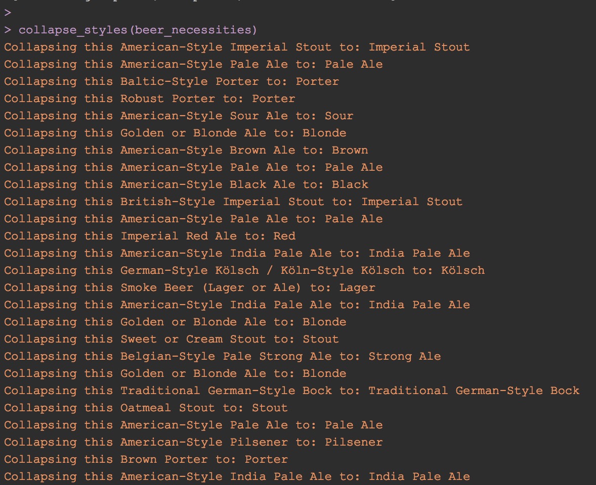
Cool, now we’ve got a factor column in our dataframe with only 28 levels instead of 170.

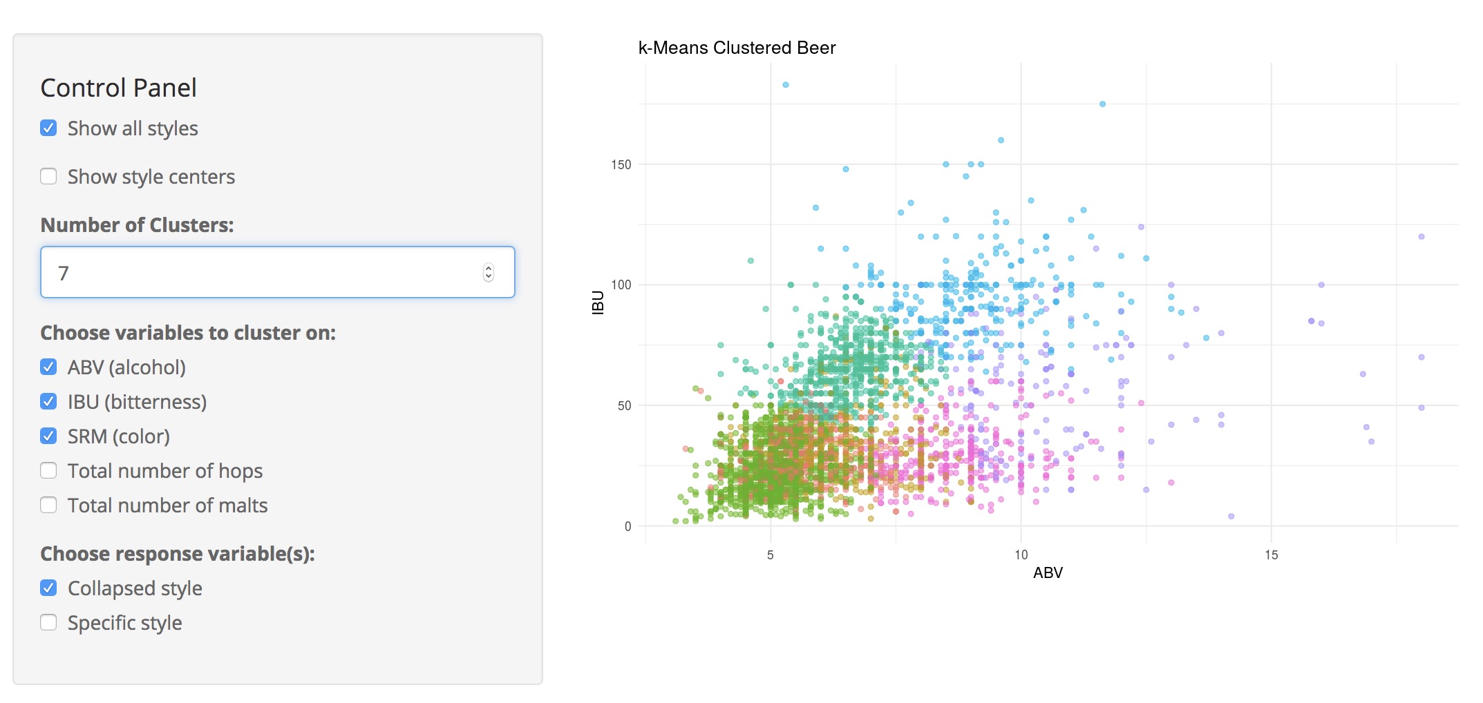
After a little time spent reading documentation, crafting a few functions for grabbing the beer data we need and getting it into a tidy data structure that’s easy to manipulate, we’re off to the races. Now’s probably a good time to crack a cold one before moving onto some actual analysis! In my case, that actual analysis mainly involved looking at clusters of beers by building this Shiny app and trying to predict a beer’s style using a random forest and a small neural net.

If you made it this far and are interested in reading more of my yammering on about the subject, my upstanding coworker Eddie, founder of the honourable Earlybird Software Open Beer Consortium, took the time to interview me about the project. Once again, all the code for the project is up at https://github.com/aedobbyn/beer-data-science. Pull requests are more than welcome.

Cheers and happy exploring!

devtools::session_info()

## Warning in as.POSIXlt.POSIXct(Sys.time()): unknown timezone 'zone/tz/2017c.
## 1.0/zoneinfo/America/Chicago'

## Session info -------------------------------------------------------------

##  setting  value                       
##  version  R version 3.3.3 (2017-03-06)
##  system   x86_64, darwin13.4.0        
##  ui       X11                         
##  language (EN)                        
##  collate  en_US.UTF-8                 
##  tz       <NA>                        
##  date     2018-02-15

## Packages -----------------------------------------------------------------

##  package    * version    date       source                          
##  assertthat   0.2.0      2017-04-11 CRAN (R 3.3.3)                  
##  backports    1.1.2      2017-12-13 cran (@1.1.2)                   
##  base       * 3.3.3      2017-03-07 local                           
##  bindr        0.1        2016-11-13 CRAN (R 3.3.3)                  
##  bindrcpp     0.2        2017-06-17 CRAN (R 3.3.3)                  
##  blogdown     0.5        2018-01-24 CRAN (R 3.3.3)                  
##  bookdown     0.5        2017-08-20 cran (@0.5)                     
##  broom        0.4.3      2017-11-20 cran (@0.4.3)                   
##  cellranger   1.1.0      2016-07-27 CRAN (R 3.3.3)                  
##  codetools    0.2-15     2016-10-05 CRAN (R 3.3.3)                  
##  colorspace   1.3-2      2016-12-14 CRAN (R 3.3.3)                  
##  crayon       1.3.4      2018-02-13 Github (r-lib/crayon@95b3eae)   
##  curl         3.1        2017-12-12 CRAN (R 3.3.2)                  
##  datasets   * 3.3.3      2017-03-07 local                           
##  devtools     1.13.4     2017-11-09 cran (@1.13.4)                  
##  digest       0.6.13     2017-12-14 cran (@0.6.13)                  
##  dplyr      * 0.7.4      2017-09-28 CRAN (R 3.3.2)                  
##  emo        * 0.0.0.9000 2017-08-21 Github (hadley/emo@86af4e6)     
##  evaluate     0.10.1     2017-06-24 CRAN (R 3.3.3)                  
##  feather    * 0.3.1      2017-09-24 Github (wesm/feather@be5141b)   
##  forcats      0.2.0      2017-01-23 CRAN (R 3.3.3)                  
##  foreign      0.8-69     2017-06-21 CRAN (R 3.3.3)                  
##  ggplot2    * 2.2.1      2016-12-30 CRAN (R 3.3.2)                  
##  glue         1.2.0      2017-10-29 CRAN (R 3.3.2)                  
##  graphics   * 3.3.3      2017-03-07 local                           
##  grDevices  * 3.3.3      2017-03-07 local                           
##  grid         3.3.3      2017-03-07 local                           
##  gtable       0.2.0      2016-02-26 CRAN (R 3.3.3)                  
##  haven        1.1.0      2017-07-09 CRAN (R 3.3.3)                  
##  here       * 0.1        2017-05-28 CRAN (R 3.3.2)                  
##  highr        0.6        2016-05-09 CRAN (R 3.3.3)                  
##  hms          0.4.0      2017-11-23 CRAN (R 3.3.2)                  
##  htmltools    0.3.6      2017-04-28 CRAN (R 3.3.3)                  
##  httpuv       1.3.5.9000 2017-09-29 Github (rstudio/httpuv@2a23c0a) 
##  httr         1.3.1      2017-08-20 cran (@1.3.1)                   
##  jsonlite   * 1.5        2017-06-01 CRAN (R 3.3.3)                  
##  knitr      * 1.18       2017-12-27 cran (@1.18)                    
##  lattice      0.20-35    2017-03-25 CRAN (R 3.3.3)                  
##  lazyeval     0.2.1      2017-10-29 CRAN (R 3.3.2)                  
##  lubridate    1.7.1      2017-11-03 cran (@1.7.1)                   
##  magrittr     1.5        2014-11-22 CRAN (R 3.3.3)                  
##  memoise      1.1.0      2018-02-01 Github (hadley/memoise@611cfad) 
##  methods    * 3.3.3      2017-03-07 local                           
##  mime         0.5        2016-07-07 CRAN (R 3.3.3)                  
##  miniUI       0.1.1      2016-01-15 CRAN (R 3.3.0)                  
##  mnormt       1.5-5      2016-10-15 CRAN (R 3.3.0)                  
##  modelr       0.1.1      2017-07-24 CRAN (R 3.3.3)                  
##  munsell      0.4.3      2016-02-13 CRAN (R 3.3.3)                  
##  nlme         3.1-131    2017-02-06 CRAN (R 3.3.3)                  
##  parallel     3.3.3      2017-03-07 local                           
##  pkgconfig    2.0.1      2017-03-21 CRAN (R 3.3.3)                  
##  plyr         1.8.4      2016-06-08 CRAN (R 3.3.3)                  
##  psych        1.7.8      2017-09-09 CRAN (R 3.3.3)                  
##  purrr      * 0.2.4      2017-10-18 CRAN (R 3.3.2)                  
##  R6           2.2.2      2017-06-17 CRAN (R 3.3.3)                  
##  Rcpp         0.12.14    2017-11-23 cran (@0.12.14)                 
##  readr      * 1.1.1      2017-05-16 CRAN (R 3.3.3)                  
##  readxl       1.0.0      2017-04-18 CRAN (R 3.3.3)                  
##  reshape2     1.4.3      2017-12-11 cran (@1.4.3)                   
##  rlang        0.1.6.9003 2018-02-13 Github (r-lib/rlang@616fd4d)    
##  rmarkdown    1.8        2017-11-17 cran (@1.8)                     
##  rprojroot    1.3-2      2018-01-03 cran (@1.3-2)                   
##  rvest        0.3.2      2016-06-17 CRAN (R 3.3.0)                  
##  scales       0.5.0.9000 2017-11-04 Github (hadley/scales@d767915)  
##  shiny        1.0.5.9000 2017-11-20 Github (rstudio/shiny@cad20a0)  
##  stats      * 3.3.3      2017-03-07 local                           
##  stringi      1.1.6      2017-11-17 CRAN (R 3.3.2)                  
##  stringr      1.2.0      2017-02-18 CRAN (R 3.3.3)                  
##  tibble     * 1.3.4      2017-08-22 cran (@1.3.4)                   
##  tidyr      * 0.7.2      2017-10-16 cran (@0.7.2)                   
##  tidyverse  * 1.1.1      2017-01-27 CRAN (R 3.3.3)                  
##  tools        3.3.3      2017-03-07 local                           
##  utils      * 3.3.3      2017-03-07 local                           
##  withr        2.1.1.9000 2017-12-26 Github (jimhester/withr@df18523)
##  xfun         0.1        2018-01-22 CRAN (R 3.3.3)                  
##  xml2         1.1.1      2017-01-24 cran (@1.1.1)                   
##  xtable       1.8-2      2016-02-05 CRAN (R 3.3.3)                  
##  yaml         2.1.16     2017-12-12 cran (@2.1.16)